Page 309 -

TRANSPORTATION SIMPLEX METHOD: A SPECIAL-PURPOSE SOLUTION PROCEDURE 289

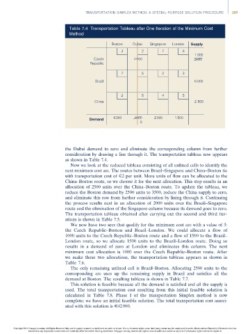
Table 7.4 Transportation Tableau after One Iteration of the Minimum Cost
Method

Boston Dubai Singapore London Supply
3 2 7 6
1 000
Czech 4 000 5000
Republic

7 5 2 3
Brazil 6 000

2 5 4 5
China 2 500

Demand 6 000 4000 2 000 1 500
0

the Dubai demand to zero and eliminate the corresponding column from further
consideration by drawing a line through it. The transportation tableau now appears
as shown in Table 7.4.
Now we look at the reduced tableau consisting of all unlined cells to identify the
next minimum cost arc. The routes between Brazil–Singapore and China–Boston tie
with transportation cost of E2 per unit. More units of flow can be allocated to the
China–Boston route, so we choose it for the next allocation. This step results in an
allocation of 2500 units over the China–Boston route. To update the tableau, we
reduce the Boston demand by 2500 units to 3500, reduce the China supply to zero,
and eliminate this row from further consideration by lining through it. Continuing
the process results next in an allocation of 2000 units over the Brazil–Singapore
route and the elimination of the Singapore column because its demand goes to zero.
The transportation tableau obtained after carrying out the second and third iter-
ations is shown in Table 7.5.
We now have two arcs that qualify for the minimum cost arc with a value of 3:
the Czech Republic–Boston and Brazil–London. We could allocate a flow of
1000 units to the Czech Republic–Boston route and a flow of 1500 to the Brazil–
London route, so we allocate 1500 units to the Brazil–London route. Doing so
results in a demand of zero at London and eliminates this column. The next
minimum cost allocation is 1000 over the Czech Republic–Boston route. After
we make these two allocations, the transportation tableau appears as shown in
Table 7.6.
The only remaining unlined cell is Brazil–Boston. Allocating 2500 units to the
corresponding arc uses up the remaining supply in Brazil and satisfies all the
demand at Boston. The resulting tableau is shown in Table 7.7.
This solution is feasible because all the demand is satisfied and all the supply is
used. The total transportation cost resulting from this initial feasible solution is
calculated in Table 7.8. Phase I of the transportation Simplex method is now
complete; we have an initial feasible solution. The total transportation cost associ-
ated with this solution is E42 000.

Copyright 2014 Cengage Learning. All Rights Reserved. May not be copied, scanned, or duplicated, in whole or in part. Due to electronic rights, some third party content may be suppressed from the eBook and/or eChapter(s). Editorial review has
deemed that any suppressed content does not materially affect the overall learning experience. Cengage Learning reserves the right to remove additional content at any time if subsequent rights restrictions require it.