Page 287 - Analysis, Synthesis and Design of Chemical Processes, Third Edition

The equations from Table 9.4 are used in Example 9.23.

Example 9.23

For the project given in Example 9.21, the manufacturing costs, excluding depreciation, are $30 million
per year, and the revenues from sales are $75 million per year. Given the depreciation values calculated
in Example 9.21, calculate the following for a 10-year period after start-up of the plant.
a. The after-tax profit (net profit)
b. The after-tax cash flow, assuming a taxation rate of 30%
6
From Equations (9.27) and (9.28) (all numbers are in $10 ),
After-tax profit = (75 – 30 – d )(1–0.3) = 31.5 – (0.7)(d )
k
k
After-tax cash flow = (75 – 30 – d )(1 – 0.3) + d = 31.5 + (0.3)(d )
k
k
k
A sample calculation for year 1 (k = 1) is provided:
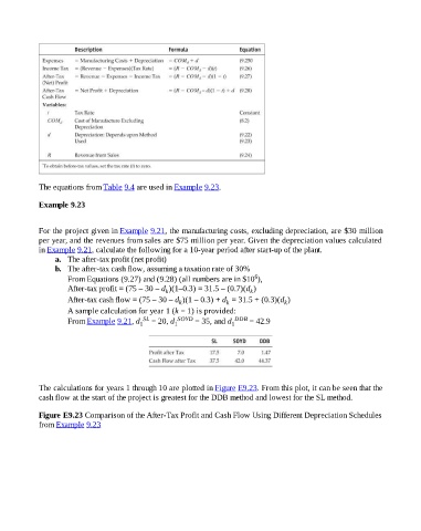
From Example 9.21, d 1 SL = 20, d 1 SOYD = 35, and d 1 DDB = 42.9

The calculations for years 1 through 10 are plotted in Figure E9.23. From this plot, it can be seen that the
cash flow at the start of the project is greatest for the DDB method and lowest for the SL method.

Figure E9.23 Comparison of the After-Tax Profit and Cash Flow Using Different Depreciation Schedules
from Example 9.23