Page 427 - Analysis, Synthesis and Design of Chemical Processes, Third Edition

mole fraction of i, is the fugacity coefficient of pure i at its vapor pressure at T, and is the molar
volume of pure liquid i at T.

The roles of the terms in Equation (13.1) are discussed in detail in standard thermodynamics texts. Here,
it is sufficient to point out that the two terms closest to the equal sign (on either side of the equal sign)
give Raoult’s Law and that the most important of the remaining correction terms is usually γ , the activity
i
coefficient. Thus, use of an activity-coefficient model requires values for the pure-component vapor
pressures at the temperature of the system. There are several important considerations in using activity-
coefficient models.
• If no BIPs are available for a given binary system, an activity-coefficient model will give results
similar to but not necessarily the same as those for an ideal solution.
• The standard version of the Wilson equation cannot predict liquid-liquid immiscibility.
• The BIPs for various activity-coefficient models can be estimated by UNIFAC. However, caution
must be exercised because increased uncertainty is inserted into the model with such estimation.
• Some BIP estimation may be done automatically by the simulator.
• There are no reliable rules for choosing an activity-coefficient model a priori. The standard
procedure is to check the correlation of experimental data by several such models and then
choose the model that gives the best correlation.
• Parameters regressed from VLE data are often unreliable when used for LLE prediction (and vice
versa). Therefore, some process simulators provide a choice between two sets of parameter
sets.
• Often ternary (and higher) data are not well predicted by activity-coefficient models and BIPs.

• The BIPs are typically highly correlated. This and the empirical nature of these models lead to
similar fits to experimental data with very different values of the BIPs.

Some of these considerations are demonstrated in Examples 13.5 and 13.6.

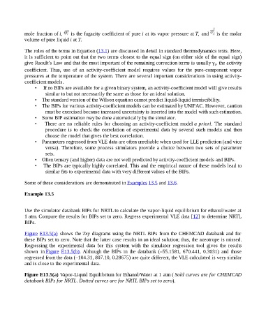
Example 13.5

Use the simulator databank BIPs for NRTL to calculate the vapor-liquid equilibrium for ethanol/water at
1 atm. Compare the results for BIPs set to zero. Regress experimental VLE data [12] to determine NRTL
BIPs.

Figure E13.5(a) shows the Txy diagrams using the NRTL BIPs from the CHEMCAD databank and for
these BIPs set to zero. Note that the latter case results in an ideal solution; thus, the azeotrope is missed.
Regressing the experimental data for this system with the simulator regression tool gives the results
shown in Figure E13.5(b). Although the BIPs in the databank (–55.1581, 670.441, 0.3031) and those
regressed from the data (–104.31, 807.10, 0.28675) are quite different, the VLE calculated is very similar
and is close to the experimental data.

Figure E13.5(a) Vapor-Liquid Equilibrium for Ethanol/Water at 1 atm ( Sold curves are for CHEMCAD
databank BIPs for NRTL. Dotted curves are for NRTL BIPs set to zero).