Page 193 - Applied Numerical Methods Using MATLAB

182 NONLINEAR EQUATIONS
and so we may be optimistic about the possibility of reaching the solution
with (E4.1.4). To confirm this, we need just a few iterations, which can
be performed by using the routine “fixpt()”.

>>gb=inline(’-((x-1).^2-3)/2’,’x’);
>>[x,err,xx]=fixpt(gb,1,1e-4,50);
>>xx
1.0000 1.5000 1.3750 1.4297 1.4077 ...
√
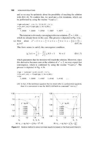
The iteration is obviously converging to the true solution 2 = 1.414 ... ,
which we already know in this case. This process is depicted in Fig. 4.1a.
2
(c) How about x = 2 → x = 2 → x + x = 2 + x → x = 1 x + 2 =
x x 2 x
g c (x)? (E4.1.6)
This form seems to satisfy the convergence condition

1 2
|g c (x)|= 1 − ≤ 0.5 < 1 ∀x ∈ I (E4.1.7)
2 x 2
which guarantees that the iteration will reach the solution. Moreover, since
2
this derivative becomes zero at the solution of x = 2, we may expect fast
convergence, which is confirmed by using the routine “fixpt()”. The
process is depicted in Fig. 4.1b.

>>gc = inline(’(x+2./x)/2’,’x’);
>>[x,err,xx] = fixpt(gc,1,1e-4,50);
>>xx
1.0000 1.5000 1.4167 1.4142 1.4142 ...

(cf) In fact, if the nonlinear equation that we must solve is a polynomial equation,
then it is convenient to use the MATLAB built-in command “roots()”.

1.55 1.55
y = x y = x
1.5 1.5
y = g (x) y = g (x)
c
b
1.45 1.45
1.0000 1.0000
1.5000 1.5000
1.4 1.3750 1.4 1.4167
1.4297 1.4142
1.4077 1.4142
1.35 1.35
1 1.2 1.4 1.6 1 1.2 1.4 1.6
x 0 x 2 x x 1 x 0 x 2 x 1
3
1
1
2
(a) x k + 1 = g (x ) = − {(x − 1) −3} (b) x k + 1 = g (x ) = x + x 2 k
k
b
k
k
k
c
2
2
Figure 4.1 Iterative method to solve nonlinear equations based on the fixed-point theorem.