Page 24 - Applied Numerical Methods Using MATLAB

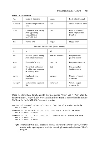
BASIC OPERATIONS OF MATLAB 13
Table 1.3 (continued)
find Index of element(s) roots Roots of polynomial

flops(0) Reset the flops count to tic Start a stopwatch timer
zero

flops Cumulative # of floating toc Read the stopwatch
point operations timer (elapsed time
(unavailable in from tic)
MATLAB 6.x)

date Present date magic Magic square
Reserved Variables with Special Meaning
√
i,j −1 pi π
eps Machine epsilon floating realmax realmin Largest/smallest
point relative accuracy positive number
break Exit while/for loop Inf, inf Largest number (∞)

end The end of for-loop or NaN Not a Number
if, while, case statement (undetermined)
or an array index

nargin Number of input nargout Number of output
arguments arguments

varargin Variable input argument varargout Variable output
list argument list

Once we store these functions into the files named ‘f1.m’ and ‘f49.m’ after the
function names, respectively, we can call and use them as needed inside another
M-file or in the MATLAB Command window.

>>f1([0 1]) %several values of a scalar function of a scalar variable
ans = 1.0000 0.1111
>>f49([0 1]) %a value of a 2-D vector function of a vector variable
ans = -1.0000 -5.5000
>>feval(’f1’,[0 1]), feval(’f49’,[0 1]) %equivalently, yields the same
ans = 1.0000 0.1111
ans = -1.0000 -5.5000

(Q5) With the function f1(x) defined as a scalar function of a scalar variable, we enter
a vector as its input argument to obtain a seemingly vector-valued output. What’s
going on?