Page 22 - Applied Numerical Methods Using MATLAB

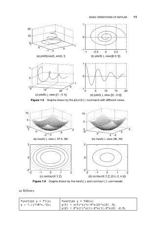
BASIC OPERATIONS OF MATLAB 11
1
20
10 0

0
1 1
0 0
−1 −1 −1
−1 −0.5 0 0.5 1
(a) plot3(cos(t), sin(t), t) (b) plot3( ), view([0 0 1])
1
1

0
0
1
−1 0
0 10 −1 −1
20 0 5 10 15 20
(c) plot3( ), view [(1 −3 1)] (d) plot3( ), view ([0 −3 0])
Figure 1.5 Graphs drawn by the plot3() command with different views.

10 10
5
5
0
2 2 0 2
0 0 −2 0
−2 −2 0 2 −2
(a) mesh( ), view (−37.5, 30) (b) mesh( ), view (30, 20)
2 2

0 0

−2 −2
−2 −1 0 1 2 −2 −1 0 1 2
(c) contour(X,Y,Z) (d) contour(X,Y,Z, [0.5, 2, 4.5])
Figure 1.6 Graphs drawn by the mesh() and contour() commands.

as follows.

function y = f1(x) function y = f49(x)
y = 1./(1+8*x.^2); y(1) = x(1)*x(1)+4*x(2)*x(2) -5;
y(2) = 2*x(1)*x(1)-2*x(1)-3*x(2) -2.5;