Page 18 - Applied Numerical Methods Using MATLAB

BASIC OPERATIONS OF MATLAB 7
(A2) >>axis([10 20 0 30]), grid on
>>plot(days,temp)
(Q3) How do we make the scales of the horizontal/vertical axes equal so that a circle
appears round, not like an ellipse?
(A3) >>axis(’equal’)
(Q4) How do we have another graph overlapped onto an existing graph?
(A4) If you use the ‘hold on’ command after plotting the first graph, any following
graphs in the same section will be overlapped onto the existing one(s) rather
than plotted newly. For example:

>>hold on, plot(days,temp(:,1),’b*’, days,temp(:,2),’ro’)
This will be good until you issue the command ‘hold off’ or clear all the graphs
in the graphic window by using the ‘clf’ command.

Sometimes we need to see the interrelationship between two variables. Sup-
pose we want to plot the lowest/highest temperature, respectively, along the
horizontal/vertical axis in order to grasp the relationship between them. Let us
try using the following command:
>>plot(temp(:,1),temp(:,2),’kx’) % temp(:,2) vs. temp(:,1) in black ’x’

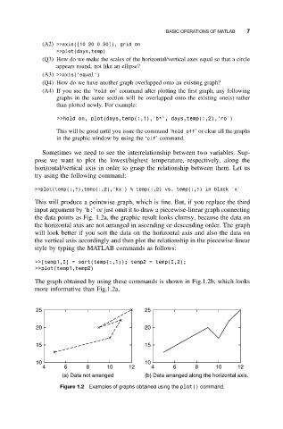
This will produce a pointwise graph, which is fine. But, if you replace the third
input argument by ‘b:’ or just omit it to draw a piecewise-linear graph connecting
the data points as Fig. 1.2a, the graphic result looks clumsy, because the data on
the horizontal axis are not arranged in ascending or descending order. The graph
will look better if you sort the data on the horizontal axis and also the data on
the vertical axis accordingly and then plot the relationship in the piecewise-linear
style by typing the MATLAB commands as follows:
>>[temp1,I] = sort(temp(:,1)); temp2 = temp(I,2);
>>plot(temp1,temp2)
The graph obtained by using these commands is shown in Fig.1.2b, which looks
more informative than Fig.1.2a.

25 25

20 20

15 15

10 10
4 6 8 10 12 4 6 8 10 12
(a) Data not arranged (b) Data arranged along the horizontal axis.

Figure 1.2 Examples of graphs obtained using the plot() command.