Page 16 - Applied Numerical Methods Using MATLAB

BASIC OPERATIONS OF MATLAB 5
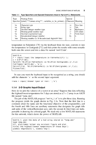
Table 1.1 Type Specifiers and Special Characters Used in fprintf() Statements
Type Printing Form: Special
Specifier fprintf(‘**format string**’, variables to be printed,..) Character Meaning
%c Character type \n New line
%s String type \t Tab
%d Decimal integer number type \b Backspace
%f Floating point number type \r CR return
%e Decimal exponential type \f Form feed
%x Hexadecimal integer number %% %
%bx Floating number in 16 hexadecimal digits(64 bits) ’’ ’

◦
temperature in Fahrenheit [ F] via the keyboard from the user, converts it into
◦
the temperature in Centigrade [ C] and then prints the results with some remarks
both onto the screen and into a data file named ‘nm113.dat’.

%nm113.m
f = input(’Input the temperature in Fahrenheit[F]:’);
c = 5/9*(f-32);
fprintf(’%5.2f(in Fahrenheit) is %5.2f(in Centigrade).\n’,f,c)
fid=fopen(’nm113.dat’, ’w’);
fprintf(fid, ’%5.2f(Fahrenheit) is %5.2f(Centigrade).\n’,f,c);
fclose(fid);

In case you want the keyboard input to be recognized as a string, you should
add the character ’s’ as the second input argument.
>>ans = input(’Answer <yes> or <no>: ’,’s’)

1.1.4 2-D Graphic Input/Output
How do we plot the value(s) of a vector or an array? Suppose that data reflecting
the highest/lowest temperatures for 5 days are stored as a 5 × 2 array in an ASCII
file named ‘temp.dat’.
The job of the MATLAB program “nm114_1.m” is to plot these data. Running
the program yields the graph shown in Fig. 1.1a. Note that the first line is a
comment about the name and the functional objective of the program(file), and
the fourth and fifth lines are auxiliary statements that designate the graph title
and units of the vertical/horizontal axis; only the second & third lines are indis-
pensable in drawing the colored graph. We need only a few MATLAB statements
for this artwork, which shows the power of MATLAB.

%nm114_1: plot the data of a 5x2 array stored in "temp.dat"
load temp.dat
clf, plot(temp) %clear any existent figure and plot
title(’the highest/lowest temperature of these days’)
ylabel(’degrees[C]’), xlabel(’day’)