Page 408 - Applied Numerical Methods Using MATLAB

PROBLEMS 397
(a) Make the above routine “eig_QR()” that uses the MATLAB built-in
routine “qr()” and then apply it to a 4 × 4 random symmetric matrix A
generated by the following MATLAB statements.

>> A = rand(4); A=A+A’;

(b) Make the above routine “eig_QR_Hs()” that transforms a given matrix
into a Hessenberg form by using the routine “Hessenberg()” (appeared
in Problem 8.5) and then repetitively makes the QR factorization by
using the routine “qr_Hessenberg()” (appeared in Problem 8.6) and
the similarity transformation by the orthogonal matrix Q until the matrix
becomes diagonal. Apply it to the 4 × 4 random symmetric matrix A
generated in (a) and compare the result with those obtained in (a) and
by using the MATLAB built-in routine “eig()” for cross-check.
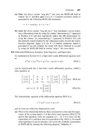
8.8 Differential/Difference Equation, State Equation, and Eigenvalue
As mentioned in Section 6.5.3, a high-order scalar differential equation such
as
(3)
(2)
x (t) + a 2 x (t) + a 1 x (t) + a 0 x(t) = u(t) (P8.8.1)

can be transformed into a first-order vector differential equation, called a
state equation, as

       
x 1 (t) 0 1 0 x 1 (t) 0
x 2 (t) 0 0 1 x 2 (t) 0 u(t) (P8.8.2a)

  =     +  
x 3 (t) −a 0 −a 1 −a 2 x 3 (t) 1

 
x 1 (t)
x(t) = [ 10 0 ]  x 2 (t)  (P8.8.2b)
x 3 (t)
The characteristic equation of the differential equation (P8.8.1) is

3
2
s + a 2 s + a 1 s + a 0 = 0 (P8.8.3)
and its roots are called the characteristic roots.
(a) What is the relationship between these characteristic roots and the eigen-
values of the system matrix A of the above state equation (P8.8.2)? To
answer this question, write the equation |λI − A|= 0 to solve for the
eigenvalues of A, and show that it is equivalent to Eq. (P8.8.3). To extend
your experience or just for practice, you can try the symbolic computation
of MATLAB by running the following program “nm8p08a.m”.