Page 455 - Applied Numerical Methods Using MATLAB

444 PARTIAL DIFFERENTIAL EQUATIONS
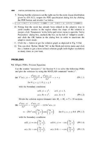
9. Noting that the solution is not the right one for the point charge distribution
given by (E9.10.2), reopen the PDE specification dialog box by clicking
the PDE button and rewrite f as below.
, , , ,
10. Noting that the mesh has already been refined in the adaptive way to
yield smaller meshes in the region where the slope of the solution is
steeper, click ‘Parameters’ in the Solve pull-down menu to open the ‘Solve
Parameters’ dialog box, uncheck the box on the left of ‘Adaptive mode’,
and click the OK button in the dialog box in order to inactivate the
adaptive mesh mode.
11. Click the = button to get the solution graph as depicted in Fig. 9.16d.
∧
12. You can click ‘Refine Mesh( M)’ in the Mesh pull-down menu and click
the = button to get a more refined solution graph (with higher resolution)
as many times as you want.

PROBLEMS

9.1 Elliptic PDEs: Poisson Equations
Use the routine “poisson()” (in Section 9.1) to solve the following PDEs
and plot the solutions by using the MATLAB command “mesh()”.

2
2
∂ u(x, y) ∂ u(x, y)
2
(a) ∇ u(x, y) = + = x + y (P9.1.1)
∂x 2 ∂y 2
for 0 ≤ x ≤ 1, 0 ≤ y ≤ 1
with the boundary conditions
2
u(0,y) = y , u(1,y) = 1,
2
u(x, 0) = x , u(x, 1) = 1 (P9.1.2)
Divide the solution region (domain) into M x × M y = 5 × 10 sections.

2
2
∂ u(x, y) ∂ u(x, y) 2
(b) + − 12.5π u(x, y)
∂x 2 ∂y 2
5π 5π

2
=−25π cos x cos y for 0 ≤ x, y ≤ 0.4 (P9.1.3)
2 2
with the boundary conditions
5π 5π

u(0,y) = cos y , u(0.4,y) =− cos y (P9.1.4)
2 2
5π 5π

u(x, 0) = cos x , u(x, 0.4) =− cos x (P9.1.5)
2 2