Page 453 - Applied Numerical Methods Using MATLAB

442 PARTIAL DIFFERENTIAL EQUATIONS
0:0.1:2 and the initial conditions as Eq. (E9.9.3) before clicking the =
button to solve the PDE. (See Fig. 9.15b.)
6. Do almost the same thing as step 6 for the case of parabolic PDE in
Example 9.8.

Finally, you could see the solution graphs like Figs. 9.15(d1)&(d2), that are
similar to Figs. 9.6(a)&(c).

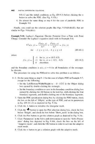
Example 9.10. Laplace’s Equation: Electric Potential Over a Plate with Point
Charge. Consider the Laplace’s equation (dealt with in Example 9.6)
2
2
∂ u(x, y) ∂ u(x, y)
2
∇ u(x, y) = + = f (x, y)
∂x 2 ∂y 2
for −1 ≤ x ≤+1, −1 ≤ y ≤+1 (E9.10.1)
where

 −1for (x, y) = (0.5, 0.5)
f (x, y) = +1for (x, y) = (−0.5, −0.5) (E9.10.2)
0 elsewhere

and the boundary condition is u(x, y) = 0 for all boundaries of the rectangu-
lar domain.
The procedure for using the PDEtool to solve this problem is as follows.

0–2. Do the same thing as step 0–2 for the case of elliptic PDE in Example 9.7,
except for the following.
ž Set the Left/Bottom/Width/Height to −1/−1/2/2 in the Object dialog
box opened by double-clicking the rectangle.
ž Set the boundary condition to zero in the boundary condition dialog box
opened by clicking the ∂ button in the tool-bar, shift-clicking the four
boundary segments, and double-clicking one of the boundary segments.
3. Open the PDE specification dialog box by clicking the PDE button, check
the box on the left of ‘Elliptic’ as the type of PDE, and set its parameters
in Eq. (E9.10.1,2) as depicted in Fig. 9.16a.
4. Click the button to initialize the triangular mesh.
5. Click the button to open the Plot selection dialog box, check the box
before ‘Height’, and check the box before ‘Show mesh’ in the dialog box.
6. Click the Plot button to get the solution graph as depicted in Fig. 9.16c.
7. Click ‘Parameters’ in the Solve pull-down menu to open the ‘Solve Param-
eters’ dialog box depicted in Fig. 9.16b, check the box on the left of
‘Adaptive mode’, and click the OK button in order to activate the adaptive
mesh mode.
8. Click the = button to get a solution graph with the adaptive mesh.