Page 73 - Applied Numerical Methods Using MATLAB

62 MATLAB USAGE AND COMPUTATIONAL ERRORS

function y = zeroing(x,M,m)
%zero out every (kM - m)th element
if nargin < 3, m = 0; end
if M<=0,M=1; end
m = mod(m,M);
Nx = length(x); N = floor(Nx/M);
y = x; y(M*[1:N] - m) = 0;

(g) Make a MATLAB routine “sampling(x,M,m)”, which samples every
(kM-m)th element of a given row vector sequence x to makeanew
sequence. Write a MATLAB statement to apply the routine for sampling
every (3k − 2)th element of x = [ 137 249 ]toget

y = [1 2]

(h) Make a MATLAB routine ‘rotation_r(x,M)”, which rotates a given
row vector sequence x right by M samples, say, making rotate_r([1
2 3 4 5],3) = [34512].
1.16 Distribution of a Random Variable: Histogram
Make a routine randu(N,a,b), which uses the MATLAB function rand()
to generate an N-dimensional random vector having the uniform distribution
over [a, b] and depicts the graph for the distribution of the elements of
the generated vector in the form of histogram divided into 20 sections as
Fig.1.7. Then, see what you get by typing the following statement into the
MATLAB command window.

>>randu(1000,-2,2)

What is the height of the histogram on the average?
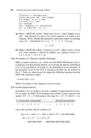
1.17 Number Representation
In Section 1.2.1, we looked over how a number is represented in 64 bits.
For example, the IEEE 64-bit floating-point number system represents the
1
2
1
2
number 3(2 ≤ 3 < 2 ) belonging to the range R 1 = [2 , 2 ) with E = 1as
0 100 0000 0000 1000 0000 0000 . . . . . . . . . . . . 0000 0000 0000 0000 0000
4 0 0 8 0 0 . . . . . . . . 0 0 0 0 0

where the exponent and the mantissa are
Exp = E + 1023 = 1 + 1023 = 1024 = 2 10 = 100 0000 0000

M = (3 × 2 −E − 1) × 2 52 = 2 51
= 1000 0000 0000 .... 0000 0000 0000 0000 0000