Page 100 - Applied Probability

5. Genetic Identity Coefficients
84
algorithm just given for the computation of kinship coefficients [13]. We
will explore more recent algorithms that approach the problem of com-
puting identity coefficients obliquely by first defining generalized kinship
coefficients and then relating these generalized kinship coefficients to the
pairwise identity coefficients [9].
i’s genes g i 1 g i 2
j’s genes g 1 g 2
j j

S ∗ 1 S ∗ 2 S ∗ 3 S ∗ 4 S ∗ 5

S ∗ 6 S ∗ 7 S ∗ 8 S ∗ 9 S 10
∗

∗
∗
∗
∗
∗
S 11 S 12 S 13 S 14 S 15
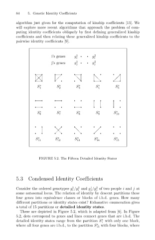
FIGURE 5.2. The Fifteen Detailed Identity States

5.3 Condensed Identity Coefficients

1
2
1
2
Consider the ordered genotypes g /g and g /g of two people i and j at
i
j
i
j
some autosomal locus. The relation of identity by descent partitions these
four genes into equivalence classes or blocks of i.b.d. genes. How many
different partitions or identity states exist? Exhaustive enumeration gives
a total of 15 partitions or detailed identity states.
These are depicted in Figure 5.2, which is adapted from [6]. In Figure
5.2, dots correspond to genes and lines connect genes that are i.b.d. The
detailed identity states range from the partition S with only one block,
∗
1
where all four genes are i.b.d., to the partition S 15 with four blocks, where
∗