Page 99 - Applied Probability

83
5. Genetic Identity Coefficients
1
individual i is a founder, then set Φ ii = , reflecting the assumption that
2
founders are not inbred. For each previously considered person j, also set
Φ ij =Φ ji = 0, reflecting the fact that j can never be a descendant of i due
to our numbering convention. If i is not a founder, then let i have parents k
1
and l. It is clear that Φ ii =
2 1 + Φ kl because in sampling the genes of i we
2
are equally likely to choose either the same gene twice or both maternally
1
and paternally derived genes once. Likewise, Φ ij =Φ ji = 1 Φ jk + Φ jl
2 2
because we are equally likely to compare either the maternal gene of i or the
paternal gene of i to a randomly drawn gene from j. These rules increase
the extent of Φ by an additional diagonal entry and the corresponding
partial row and column up to the diagonal entry. This recursive process is
repeated until the matrix Φ is fully defined.
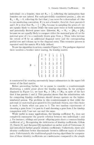
To see the algorithm in action, consider Figure 5.1. The pedigree depicted
there involves a brother–sister mating. Its kinship matrix
 
1 0 1 1 1 1
2 4 4 4 4
 1 1 1 1 
 0 2 4 4 4 1 
 4 

 1 1 1 1 3 3 

 4 4 2 4 8 8 
Φ=  
 1 1 1 1 3 3 
 4 4 4 2 8 8 
 1 1 3 3 5 3 


 4 4 8 8 8 8 
1 1 3 3 3 5
4 4 8 8 8 8
is constructed by creating successively larger submatrices in the upper left
corner of the final matrix.
Before proceeding further, let us pause to consider a counterexample
illustrating a subtle point about the kinship algorithm. In the pedigree
1
displayed in Figure 5.1, we have Φ 35 = 1 Φ 15 + Φ 25 in spite of the fact
2 2
that 3 has parents 1 and 2. This paradox shows that the substitution rule
for computing kinship coefficients should always operate on the higher-
numbered person. The problem in this counterexample is that while the
paternal (or maternal) gene passed to 3 is randomly chosen, once this choice
is made, it limits what can pass to 5. The two random experiments of
choosing a gene from 1 to pass to 3 and choosing a gene from 1 for kinship
comparison with 5 are not one and the same.
While useful in many applications, the kinship coefficient Φ ij does not
completely summarize the genetic relation between two individuals i and
j. For instance, siblings and parent–offspring pairs share a common kinship
1
coefficient of . Recognizing the deficiencies of kinship coefficients, Gillois
4
[2], Harris [3], and Jacquard [5] capitalized on earlier work of Cotterman [1]
and introduced further genetic identity coefficients. Collectively, these new
identity coefficients better discriminate between different types of relative
pairs. Unfortunately, the traditional graph-tracing algorithms for computa-
tion of these identity coefficients are cumbersome compared to the simple