Page 191 - Applied Probability

9. Descent Graph Methods
176

1
2

5
6
3
4
2/4 1/2 1/4 1/3
1/1
2/4

7 8 9 10
1/4 1/4 1/2 3/4
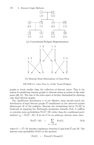
(a) Conventional Pedigree Representation
12 1 4

42 13

(b) Descent State Description of Gene Flow
FIGURE 9.1. Gene Flow in a Fully Typed Pedigree
graphs is much smaller than the collection of descent states. This is the
reason for preferring descent graphs to descent states as points of the state
space [40, 41]. The size of the state space is further diminished by allowing
only legal descent graphs.
The equilibrium distribution π of our Markov chain should match the
distribution of legal descent graphs G conditioned on the observed marker
0
phenotypes M of the pedigree. Because the normalizing factor Pr(M)is
irrelevant in applying the Metropolis acceptance formula (9.6), it suffices
to calculate joint probabilities Pr(G∩M) rather than the conditional prob-
0
abilities π =Pr(G | M). If we let G be an arbitrary descent state, then
0
0 G

Pr(G ∩ M)= Pr(G), (9.8)
0
G à 0 G∩M
where G ø G∩M denotes consistency between G and both G and M. The
0
0
descent state probability Pr(G) is the product
Pr(G) = Prior(G) Trans(G)