Page 196 - Applied Probability

181
9. Descent Graph Methods
of the next three vectors (a A ,a C ,a E )= (1, 2, 2), (a A ,a C ,a E )= (1, 2, 3),
and (a A ,a C ,a E )=(1, 2, 4) as inconsistent, backtrack to the partial vector
(a A ,a C , )= (1, 3), which is inconsistent, and so forth, until ultimately we
identify the second compatible vector (a A ,a C ,a E )=(2, 1, 2) and reject all
other allele vectors. The virtue of backtracking is that it eliminates large
numbers of incompatible vectors without actually visiting each of them.
If penetrances are quantitative, so that every genotype is compatible with
every phenotype, then S i expands to a Cartesian product having n |C i| ele-
ments, where |C i | is the number of founder genes in C i and n is the number
of alleles at the current locus. In this case, backtracking will successfully
construct every allele vector in the Cartesian product, but the correspond-
ing computational complexity balloons to unacceptable levels if either |C i |
or n is very large. Backtracking is certainly possible in small pedigrees for
recessive disease loci with just two alleles [18].
9.6 The Descent Graph Markov Chain

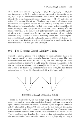
The set of descent graphs over a pedigree becomes a Markov chain if we
incorporate transition rules for moving between descent graphs. The most
basic transition rule, which we call rule T 0 , switches the origin of an arc
descending from a parent to a child from the parental maternal node to
the parental paternal node or vice versa [23, 24, 32, 40, 41]. The arbitrary
arc chosen is determined by a combination of child, locus, and maternal or
paternal source. Figure 9.3 illustrates rule T 0 at the black node.

FIGURE 9.3. Example of Transition Rule T 0
From the basic rule T 0 we can design composite transition rules that
make more radical changes in an existing descent graph and consequently
speed up the circulation of the chain. For example, the composite transition
rule T 1 illustrated in Figure 9.4 operates on the two subtrees descending
from the person with black nodes at the given locus. One of these subtrees
is rooted at the maternal node, and the other is rooted at the paternal node.
The two subtrees are detached from their rooting nodes and rerooted at
the opposite nodes. More formally, transition rule T 1 begins by choosing a