Page 24 - Applied Probability

1. Basic Principles of Population Genetics
1
1
1
1
=
q n−1 + r n−1 −
2
3
3
2
2
2
1
1
= − q n−1 + p
2
2
1
= − (q n−1 − p) . 3 2 q n−1 + r n−1 + p 7
2
Continuing in this manner,
n
1
q n − p = − (q 0 − p).
2
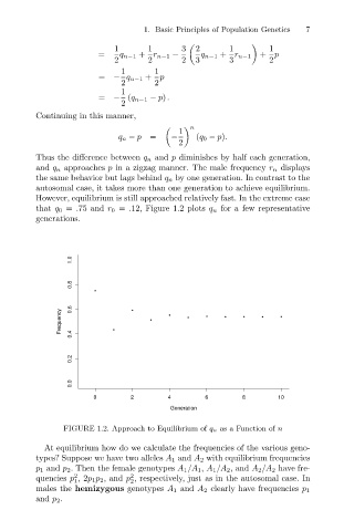
Thus the difference between q n and p diminishes by half each generation,
and q n approaches p in a zigzag manner. The male frequency r n displays
the same behavior but lags behind q n by one generation. In contrast to the
autosomal case, it takes more than one generation to achieve equilibrium.
However, equilibrium is still approached relatively fast. In the extreme case
that q 0 = .75 and r 0 = .12, Figure 1.2 plots q n for a few representative
generations.
1.0
0.8
•
Frequency 0.6 0.4 • • • • • • • • • •
0.2

0.0
0 2 4 6 8 10
Generation

FIGURE 1.2. Approach to Equilibrium of q n as a Function of n

At equilibrium how do we calculate the frequencies of the various geno-
types? Suppose we have two alleles A 1 and A 2 with equilibrium frequencies
p 1 and p 2 . Then the female genotypes A 1 /A 1 , A 1 /A 2 , and A 2 /A 2 have fre-
2
2
quencies p ,2p 1p 2 , and p , respectively, just as in the autosomal case. In
1
2
males the hemizygous genotypes A 1 and A 2 clearly have frequencies p 1
and p 2 .