Page 26 - Applied Probability

1. Basic Principles of Population Genetics
.
.
.
n
=(1 − θ) [P 0 (A i B j ) − p i q j ].
Thus, P n (A i B j ) converges to p i q j at the geometric rate 1 − θ. For two
loci on different chromosomes, the deviation from linkage equilibrium is
halved each generation. Equilibrium is approached much more slowly for 9
closely spaced loci. Similar, but more cumbersome, proofs of convergence to
linkage equilibrium can be given for three or more loci [1, 5, 9, 11]. Problem
7 explores the case of three loci.
1.5 Selection
The simplest model of evolution involves selection at an autosomal locus
with two alleles A 1 and A 2 . At generation n, let allele A 1 have population
frequency p n and allele A 2 population frequency q n =1 − p n . Under the
usual assumptions of genetic equilibrium, we deduced the Hardy-Weinberg
and linkage equilibrium laws. Now suppose that we relax the assumption of
no selection by postulating different fitnesses w A 1 /A 1 , w A 1 /A 2 , and w A 2 /A 2
for the three genotypes. Fitness is a technical term dealing with the repro-
ductive capacity rather than the longevity of people with a given genotype.
is the ratio of the expected genetic contribution to
Thus, w A 1 /A 1 /w A 1 /A 2
the next generation of an A 1 /A 1 individual to the expected genetic con-
tribution of an A 1 /A 2 individual. Since only fitness ratios are relevant,
=1 − r, and
we can without loss of generality put w A 1 /A 2 =1, w A 1 /A 1
=1 − s, provided of course that r ≤ 1 and s ≤ 1. Observe that r
w A 2 /A 2
and s can be negative.
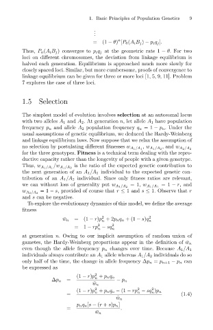
To explore the evolutionary dynamics of this model, we define the average
fitness
2
¯ w n =(1 − r)p +2p nq n +(1 − s)q 2 n
n
2
=1 − rp − sq 2 n
n
at generation n. Owing to our implicit assumption of random union of
gametes, the Hardy-Weinberg proportions appear in the definition of ¯ w n
even though the allele frequency p n changes over time. Because A 1 /A 1
individuals always contribute an A 1 allele whereas A 1 /A 2 individuals do so
only half of the time, the change in allele frequency ∆p n = p n+1 − p n can
be expressed as
2
(1 − r)p + p n q n
n
=
∆p n − p n
¯ w n
2 2 2
(1 − r)p + p n q n − (1 − rp − sq )p n
n
n
n
= (1.4)
¯ w n
p n q n [s − (r + s)p n ]
= .
¯ w n