Page 259 - Applied Probability

11. Radiation Hybrid Mapping
246
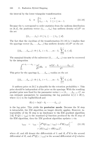
the interval by the lower triangular transformation
,
i =0
t 1
(11.18)
=
δ i
1 ≤ i ≤ m − 1.
t i+1 − t i
Because the t i correspond to order statistics from the uniform distribution
on [0,d], the positions vector (t 1 ,... ,t m ) has uniform density m!/d m on
the set
{(t 1 ,...,t m ):0 ≤ t 1 ≤· · · ≤ t m ≤ d}.
The fact that the Jacobian of the transformation (11.18) is 1 implies that
the spacings vector (δ 0 ,... ,δ m−1 ) has uniform density m!/d m on the set
m−1

{(δ 0 ,... ,δ m−1 ): 0 ≤ δ i ,i =0,... ,m − 1, δ i ≤ d}.
i=0
The marginal density of the subvector (δ 1 ,...,δ m−1 ) can now be recovered
by the integration
m! m!(d − δ 1 −· · · − δ m−1 )
d−δ 1 −···−δ m−1

dδ 0 = m .
m
d d
0
This prior for the spacings δ 1 ,...,δ m−1 resides on the set
m−1

{(δ 1 ,... ,δ m−1 ): 0 ≤ δ i ,i =1,... ,m − 1, δ i ≤ d}.
i=1
A uniform prior on [0,1] is plausible for the retention probability r. This
prior should be independent of the prior on the spacings. With the resulting
t
product prior now fixed for the parameter vector γ =(δ 1 ,...,δ m−1 ,r) ,we
can estimate parameters by maximizing the log posterior L(γ)+ R(γ),
where L(γ) is the loglikelihood and
R(γ)= ln(d − δ 1 −· · · − δ m−1 )
is the log prior. This yields the posterior mode. Because the M step
is intractable, the EM algorithm no longer directly applies. However, in-
tractability of the M step is no hindrance to the EM gradient algorithm
[13]. If Q(γ | γ old ) is the standard Q function produced by the E step of
the EM algorithm, then the EM gradient algorithm updates γ via
−1

2
20
= γ old − d Q(γ old | γ old )+ d R(γ old ) (11.19)
γ new
t
× [dL(γ old)+ dR(γ old )] ,
2
where dL and dR denote the differentials of L and R, d R is the second
20
differential of R, and d Q(γ | γ old ) is the second differential of Q relative