Page 113 - Applied Statistics And Probability For Engineers

PQ220 6234F.Ch 03 13/04/2002 03:19 PM Page 91

3-9 POISSON DISTRIBUTION 91

1.0 1.0
λ λ
0.1 2
0.8 0.8

0.6 0.6
f(x) f(x)
0.4 0.4

0.2 0.2

0 0
0 1 2 3 4 5 6 7 8 9 10 11 12
0 1 2 3 4 5 6 7 8 9 10 11 12
x
x
(a)
(b)
1.0
λ
5
0.8

0.6
f(x)
0.4

0.2

0
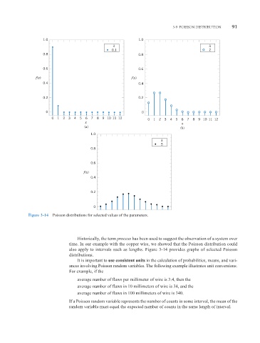
Figure 3-14 Poisson distributions for selected values of the parameters.

Historically, the term process has been used to suggest the observation of a system over
time. In our example with the copper wire, we showed that the Poisson distribution could
also apply to intervals such as lengths. Figure 3-14 provides graphs of selected Poisson
distributions.
It is important to use consistent units in the calculation of probabilities, means, and vari-
ances involving Poisson random variables. The following example illustrates unit conversions.
For example, if the
average number of flaws per millimeter of wire is 3.4, then the
average number of flaws in 10 millimeters of wire is 34, and the
average number of flaws in 100 millimeters of wire is 340.
If a Poisson random variable represents the number of counts in some interval, the mean of the
random variable must equal the expected number of counts in the same length of interval.