Page 152 - Applied Statistics And Probability For Engineers

c04.qxd 6/23/02 7:38 PM Page 130 RK UL 6 RK UL 6:Desktop Folder:

130 CHAPTER 4 CONTINUOUS RANDOM VARIABLES AND PROBABILITY DISTRIBUTIONS

2.0

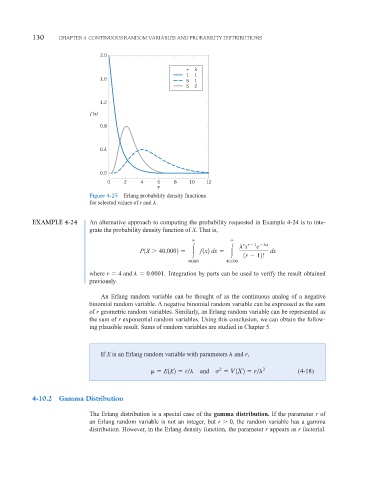
r λ
1 1
1.6
5 1
5 2
1.2
f (x)

0.8

0.4

0.0
0 2 4 6 8 10 12
x
Figure 4-25 Erlang probability density functions
for selected values of r and .

EXAMPLE 4-24 An alternative approach to computing the probability requested in Example 4-24 is to inte-
grate the probability density function of X. That is,

x e
r r 1 x
P1X 40,0002 f 1x2 dx dx
1r 12!
40,000 40,000
where r 4 and 0.0001. Integration by parts can be used to verify the result obtained
previously.

An Erlang random variable can be thought of as the continuous analog of a negative
binomial random variable. A negative binomial random variable can be expressed as the sum
of r geometric random variables. Similarly, an Erlang random variable can be represented as
the sum of r exponential random variables. Using this conclusion, we can obtain the follow-
ing plausible result. Sums of random variables are studied in Chapter 5.

If X is an Erlang random variable with parameters and r,
2
E1X2 r and V1X2 r 2 (4-18)

4-10.2 Gamma Distribution

The Erlang distribution is a special case of the gamma distribution. If the parameter r of
an Erlang random variable is not an integer, but r 0 , the random variable has a gamma
distribution. However, in the Erlang density function, the parameter r appears as r factorial.