Page 112 - Applied statistics and probability for engineers

90 Chapter 3/Discrete Random Variables and Probability Distributions

0.12
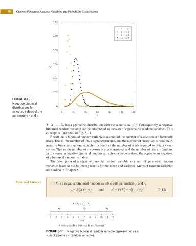
r p
5 0.1
0.10 5 0.4
10 0.4

0.08

0.06
f (x)

0.04

0.02

FIGURE 3-10
Negative binomial
distributions for 0
selected values of the 0 20 40 60 80 100 120
parameters r and p. x

X , X ,… , X r has a geometric distribution with the same value of p. Consequently, a negative
1
2
binomial random variable can be interpreted as the sum of r geometric random variables. This
concept is illustrated in Fig. 3-11.
Recall that a binomial random variable is a count of the number of successes in n Bernoulli
trials. That is, the number of trials is predetermined, and the number of successes is random. A
negative binomial random variable is a count of the number of trials required to obtain r suc-
cesses. That is, the number of successes is predetermined, and the number of trials is random.
In this sense, a negative binomial random variable can be considered the opposite, or negative,
of a binomial random variable.
The description of a negative binomial random variable as a sum of geometric random
variables leads to the following results for the mean and variance. Sums of random variables
are studied in Chapter 5.

Mean and Variance If X is a negative binomial random variable with parameters p and r,

2
E
X
μ = ( ) = r p and σ = ( ) = ( r 1 − ) p p 2 (3-12)
V X
X = X + X + X 3
2
1
X 1 X 2 X 3
1 2 3 4 5 6 7 8 9 10 11 12
Trials
indicates a trial that results in a "success."
FIGURE 3-11 Negative binomial random variable represented as a
sum of geometric random variables.