Page 109 - Applied statistics and probability for engineers

Section 3-7/Geometric and Negative Binomial Distributions 87

number of trials until the irst success. Example 3-5 analyzed successive wafers until a large

particle was detected. Then X is the number of wafers analyzed. In the transmission of bits,
X might be the number of bits transmitted until an error occurs.

Example 3-20 Digital Channel The probability that a bit transmitted through a digital transmission channel is
received in error is 0.1. Assume that the transmissions are independent events, and let the random
variable X denote the number of bits transmitted until the i rst error.
(

Then P X = ) 5 is the probability that the i rst four bits are transmitted correctly and the ifth bit is in error. This
event can be denoted as {OOOOE }, where O denotes an okay bit. Because the trials are independent and the prob-
ability of a correct transmission is 0.9,
P X = ) = ( . 4 . = .
(
P OOOOE) = 0 9 0 1 0 066
5

Note that there is some probability that X will equal any integer value. Also, if the irst trial is a success, X = 1. There-
},
fore, the range of X is {1 2 3, , ,… that is, all positive integers.
Geometric
Distribution In a series of Bernoulli trials (independent trials with constant probability p of
a success), the random variable X that equals the number of trials until the i rst
success is a geometric random variable with parameter 0 < p < 1 and
, ,…
f x ( ) = (1 − p) x−1 p x = 1 2 (3-9)

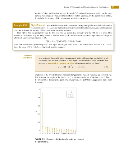
Examples of the probability mass functions for geometric random variables are shown in Fig.
(
3-9. Note that the height of the line at x is 1 − ) p times the height of the line at x − 1. That is,
the probabilities decrease in a geometric progression. The distribution acquires its name from
this result.

1.0
p
0.1
0.9
0.8

0.6

f (x)
0.4

0.2

0
0 1 2 3 4 5 6 7 8 9 1011121314151617181920
x
FIGURE 3-9 Geometric distributions for selected values of
the parameter p.