Page 104 - Applied statistics and probability for engineers

82 Chapter 3/Discrete Random Variables and Probability Distributions

⎛ n⎞
As in Example 3-16, ⎜ ⎟ equals the total number of different sequences of trials that con-
x⎠
⎝
tain x successes and n − x failures. The total number of different sequences that contain x
(
successes and n x− failures times the probability of each sequence equals P X = x).
The preceding probability expression is a very useful formula that can be applied in a num-
ber of examples. The name of the distribution is obtained from the binomial expansion. For
constants a and b, the binomial expansion is
n⎞
n
( a b) = ∑ ⎛ ⎜ ⎟ a b −
n
+
k n k
k=0 k ⎝ ⎠
Let p denote the probability of success on a single trial. Then by using the binomial expansion
with a = p and b = −1 p, we see that the sum of the probabilities for a binomial random variable

is 1. Furthermore, because each trial in the experiment is classiied into two outcomes, {success,
failure}, the distribution is called a “bi”-nomial. A more general distribution, which includes the
binomial as a special case, is the multinomial distribution, and this is presented in Chapter 5.
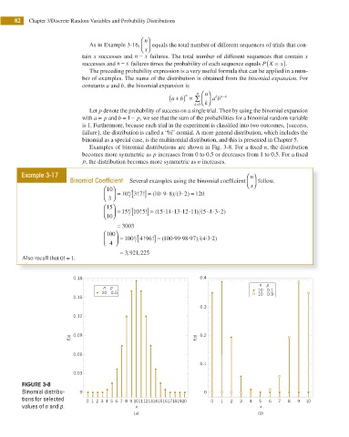
Examples of binomial distributions are shown in Fig. 3-8. For a i xed n, the distribution
becomes more symmetric as p increases from 0 to 0.5 or decreases from 1 to 0.5. For a i xed
p, the distribution becomes more symmetric as n increases.
Example 3-17 ⎛ n⎞
Binomial Coeffi cient Several examples using the binomial coefi cient ⎜ ⎟ follow.
⎝
x⎠
⎛ 10⎞
⎜ ⎝ 3 ⎠ ⎟ = 10! [ 3 7 ] =! ! ( 10 9 8) (⋅ ⋅ 3 2 =)⋅ 120
⎛ 15⎞
⎜ ⎝ 10⎠ ⎟ = 15 10 5 ] =! [ ! ! ( 15 14 13 12 11) (⋅ ⋅ ⋅ ⋅ 5 4 3 2)⋅ ⋅ ⋅

= 3003
⎛ 100⎞ . . . . .
⎜ ⎝ 4 ⎠ ⎟ = 100! [ 4 96 ] =! ! ( 100 99 98 97) ( 4 3 2)
= 3 921 225
,
,
Also recall that 0! 1= .

0.18 0.4
n p
n p
20 0.5 10 0.1
10 0.9
0.15
0.3
0.12

f(x) 0.09 f(x) 0.2

0.06
0.1
0.03

FIGURE 3-8
Binomial distribu- 0 0
tions for selected 0 1 2 3 4 5 6 7 8 9 1011121314151617181920 0 1 2 3 4 5 6 7 8 9 10
values of n and p. x x
(a) (b)