Page 105 - Applied statistics and probability for engineers

Section 3-6/Binomial Distribution 83

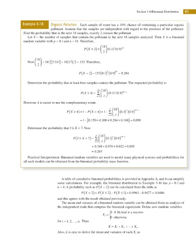
Example 3-18 Organic Pollution Each sample of water has a 10% chance of containing a particular organic
pollutant. Assume that the samples are independent with regard to the presence of the pollutant.
Find the probability that in the next 18 samples, exactly 2 contain the pollutant.
Let X = the number of samples that contain the pollutant in the next 18 samples analyzed. Then X is a binomial
random variable with p = 0.1 and n = 18. Therefore,
(
P X = ) = ⎛18 ⎞ ⎟ ( 0 1) ( 0 9) 16
2
.
2
.
⎜
⎝ 2 ⎠
⎛ 18⎞
2 16 ] = ( )
=
Now ⎜ ⎝ 2 ⎠ ⎟ = 18! [ ! ! 18 17 2 153. Therefore,
(
P X = ) = 153 ( ) ( ) =0 1. 2 0 9 16 0 284
.
.
2
Determine the probability that at least four samples contain the pollutant. The requested probability is
18 ⎛18 ⎞
x
(
9
1
0
0
P X ≥ 4 ) = ∑ ⎜ ⎟ ( . ) ( . ) 18 − x
x ⎝ x ⎠
=4
However, it is easier to use the complementary event,
(
P X ≥ ) = − ( 4 1 3 ⎛18 ⎞ ⎟ 0 1 x . 0 18 − x
P X < ) = − ∑
1
⎜
4
. ( ) ( ) 9
x ⎝ x ⎠
=0
1 [
+
+
+
= − 0 150 0.3300 0 284 0 168] = 0 098
.
.
.
.
Determine the probability that 3 ≤ X < 7. Now
(
6
=
x
0.9
P 3 ≤ X < 7) ∑ ⎛18 ⎞ ⎟ ( ) ( ) 18−x
0.1
⎜
x = 3⎝ x ⎠
+
+
+
= 0.168 0.070 0.022 0..005
= 0.265
Practical Interpretation: Binomial random variables are used to model many physical systems and probabilities for
all such models can be obtained from the binomial probability mass function.
A table of cumulative binomial probabilities is provided in Appendix A, and it can simplify
some calculations. For example, the binomial distribution in Example 3-16 has p = 0.1 and
(
n = 4. A probability such as P X = ) 2 can be calculated from the table as
(
P X = ) = ( 2 P X Ð ) = 0 9963 0 9477 = 0 0486
P X ≤ ) − (
−
.
2
1
.
.
and this agrees with the result obtained previously.
The mean and variance of a binomial random variable can be obtained from an analysis of
the independent trials that comprise the binomial experiment. Deine new random variables

⎧1 if ith trial is a success
X i = ⎨
⎩ 0 otherwise
for i = 1, 2,… , n. Then
X = X + X + … + X n
1
2
Also, it is easy to derive the mean and variance of each X i as