Page 122 - Applied statistics and probability for engineers

100 Chapter 3/Discrete Random Variables and Probability Distributions

Therefore,
11 5 11 5.
P X = ) e − . 10 = 0 113.
(
10 =
10!
Determine the probability of at least one l aw in 2 millimeters of wire. Let X denote the number of l aws in 2 mil-
limeters of wire. Then X has a Poisson distribution with
λT = 2 3 flaws/mm × 2 mm = 4 6 flaws
.
.
Therefore,
P X ≥ ) = − ( 0 1 e −4 6 . = 0 9899
(
P X = ) = −
1
.
1
Practical Interpretation: Given the assumptions for a Poisson process and a value for λ, probabilities can be calcu-

lated for intervals of arbitrary length. Such calculations are widely used to set product speciications, control processes,
and plan resources.
1.0 1.0

0.1 2
0.8 0.8

0.6 0.6

f(x) f(x)
0.4 0.4

0.2 0.2

0 0
0 1 2 3 4 5 6 7 8 9 10 11 12 0 1 2 3 4 5 6 7 8 9 10 11 12
x x
(a) (b)
1.0

5
0.8

0.6

f(x)
0.4

0.2

0
0 1 2 3 4 5 6 7 8 9 10 11 12
x
(c)

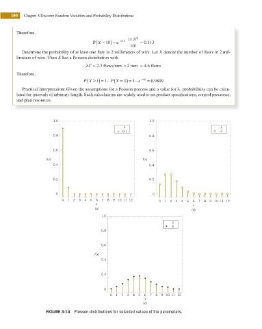
FIGURE 3-14 Poisson distributions for selected values of the parameters.