Page 123 - Applied statistics and probability for engineers

Section 3-9/Poisson Distribution 101

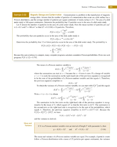
Example 3-32 Magnetic Storage and Contamination Contamination is a problem in the manufacture of magnetic
storage disks. Assume that the number of particles of contamination that occur on a disk surface has a
Poisson distribution, and the average number of particles per square centimeter of media surface is 0.1. The area of a disk
under study is 100 square centimeters. Determine the probability that 12 particles occur in the area of a disk under study.
2
Let X denote the number of particles in the area of a disk under study. Here the mean number of particles per cm
2
.
is λ = 0 1 and T = 100cm so that λT = 0 1 100. ( ) = 10 particles. Therefore,
(
P X = ) = e −10 10 12 = 0 095.
12
12!
The probability that zero particles occur in the area of the disk under study is
(
×
.
P X = ) =0 e −10 = 4 54 10 −5
Determine the probability that 12 or fewer particles occur in the area of the disk under study. The probability is
P X ≤ ) = ( 0 P X = ) + … + P X = )
(
(
P X = ) + (
12
1
12
12 e −10 ( 10) x
= ∑
x=0 x!
Because this sum is tedious to compute, many computer programs calculate cumulative Poisson probabilities. From one such
(
program, P X ≤ ) =12 0 792.
.
The mean of a Poisson random variable is
∞ e −λ T (λ T) x ∞ e −λ T (λ T) x−1
E X) = ∑ x = λ T ∑
(
x=1 x! x=1 x ( −1 )!
where the summation can start at x = 1 because the x = 0 term is zero. If a change of variable
x
y = −1 is used, the summation on the right-hand side of the previous equation is recognized
to be the sum of the probabilities of a Poisson random variable and this equals 1. Therefore,
the previous equation simplii es to
(
E X) = λ T
2
To obtain the variance of a Poisson random variable, we can start with E X ( ) and this equals
−
∞ e −λ T (λ T) x ∞ e −λ T (λ T) x 1
E X ) = ∑ x 2 = λ T ∑ x
2
(
=
=
x 1 x! x 1 x ( − 1 )!
Write x = ( x − )1 +1 to obtain
∞ e −λ T (λ T) x 1− ∞ ∞ e −λ T (λ T) x 1−
2
(
E X ) = λ T ∑ x ( − ) 1 + λ T ∑
=
=
x 1 x ( − 1 )! x 1 x ( − 1 )!
The summation in the i rst term on the right-hand side of the previous equation is recog-
2
)
nized to be the mean of X, which equals λT so that the i rst term is (λT . The summation in
the second term on the right-hand side is recognized to be the sum of the probabilities, which
equals 1. Therefore, the previous equation simplii es to E X ) = (λ T) + λ T. Because the
2
2
(
2
V X ( ) = E X ( ) −( EX) , we have
2
V X) = (λ T) + λ T − (λ T) = λ T
2
2
(
and the variance is derived.
Mean and
Variance If X is a Poisson random variable over an interval of length T with parameter λ, then
2
μ = E X) = λT and σ = V X) = λT (3-16)
(
(
The mean and variance of a Poisson random variable are equal. For example, if particle counts
follow a Poisson distribution with a mean of 25 particles per square centimeter, the variance