Page 244 - Artificial Intelligence in the Age of Neural Networks and Brain Computing

5. Deep Learning Models for EEG Signal Processing 235

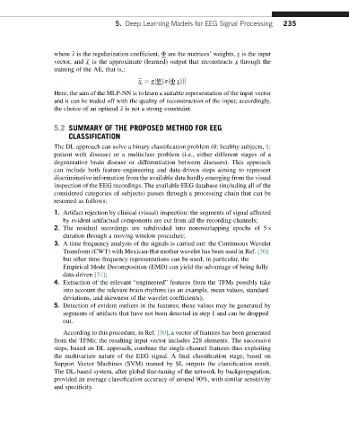
where l is the regularization coefficient, F are the matrices’ weights, x is the input
vector, and e x is the approximate (learned) output that reconstructs x through the
training of the AE, that is,:

e x ¼ s½JðsðF xÞފ
Here, the aim of the MLP-NN is to learn a suitable representation of the input vector
and it can be traded off with the quality of reconstruction of the input; accordingly,
the choice of an optimal l is not a strong constraint.

5.2 SUMMARY OF THE PROPOSED METHOD FOR EEG
CLASSIFICATION
The DL approach can solve a binary classification problem (0: healthy subjects, 1:
patient with disease) or a multiclass problem (i.e., either different stages of a
degenerative brain disease or differentiation between diseases). This approach
can include both feature-engineering and data-driven steps aiming to represent
discriminative information from the available data hardly emerging from the visual
inspection of the EEG recordings. The available EEG database (including all of the
considered categories of subjects) passes through a processing chain that can be
resumed as follows:
1. Artifact rejection by clinical (visual) inspection: the segments of signal affected
by evident artifactual components are cut from all the recording channels;
2. The residual recordings are subdivided into nonoverlapping epochs of 5 s
duration through a moving window procedure;
3. A time-frequency analysis of the signals is carried out: the Continuous Wavelet
Transform (CWT) with Mexican-Hat mother wavelet has been used in Ref. [30]
but other time-frequency representations can be used; in particular, the
Empirical Mode Decomposition (EMD) can yield the advantage of being fully
data-driven [31];
4. Extraction of the relevant “engineered” features from the TFMs possibly take
into account the relevant brain rhythms (as an example, mean values, standard
deviations, and skewness of the wavelet coefficients);
5. Detection of evident outliers in the features; these values may be generated by
segments of artifacts that have not been detected in step 1 and can be dropped
out.
According to this procedure, in Ref. [30], a vector of features has been generated
from the TFMs; the resulting input vector includes 228 elements. The successive
steps, based on DL approach, combine the single-channel features thus exploiting
the multivariate nature of the EEG signal. A final classification stage, based on
Support Vector Machines (SVM) trained by SL outputs the classification result.
The DL-based system, after global fine-tuning of the network by backpropagation,
provided an average classification accuracy of around 90%, with similar sensitivity
and specificity.