Page 35 - Artificial Intelligence in the Age of Neural Networks and Brain Computing

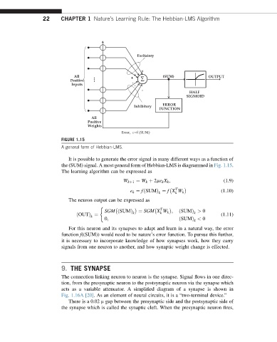
22 CHAPTER 1 Nature’s Learning Rule: The Hebbian-LMS Algorithm

Excitatory

+
+
All + (SUM) OUTPUT
Positive Â
Inputs - -
-
HALF
SIGMOID
ERROR
Inhibitory
FUNCTION
All
Positive
Weights
Error, ε=f (SUM)
FIGURE 1.15
A general form of Hebbian-LMS.

It is possible to generate the error signal in many different ways as a function of
the (SUM) signal. A most general form of Hebbian-LMS is diagrammed in Fig. 1.15.
The learning algorithm can be expressed as
W kþ1 ¼ W k þ 2me k X k ; (1.9)

T

e k ¼ fðSUMÞ ¼ f X W k (1.10)
k k
The neuron output can be expressed as
(
T
SGM ðSUMÞ k ¼ SGM X W k ; ðSUMÞ > 0
k
k
ðOUTÞ ¼ (1.11)
k
0; ðSUMÞ < 0
k
For this neuron and its synapses to adapt and learn in a natural way, the error
function f((SUM)) would need to be nature’s error function. To pursue this further,
it is necessary to incorporate knowledge of how synapses work, how they carry
signals from one neuron to another, and how synaptic weight change is effected.
9. THE SYNAPSE

The connection linking neuron to neuron is the synapse. Signal flows in one direc-
tion, from the presynaptic neuron to the postsynaptic neuron via the synapse which
acts as a variable attenuator. A simplified diagram of a synapse is shown in
Fig. 1.16A [20]. As an element of neural circuits, it is a “two-terminal device.”
There is a 0.02 m gap between the presynaptic side and the postsynaptic side of
the synapse which is called the synaptic cleft. When the presynaptic neuron fires,