Page 32 - Artificial Intelligence in the Age of Neural Networks and Brain Computing

6. Bootstrap Learning With a More “Biologically Correct” Sigmoidal Neuron 19

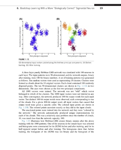
FIGURE 1.13
50-dimensional input vectors plotted along the first two principal components. (A) Before
training. (B) After training.

A three-layer purely Hebbian-LMS network was simulated with 100 neurons in
each layer. The input patterns were 50-dimensional, and the network outputs, binary
after training, were 100-bit binary numbers. A set of training patterns was generated
as follows. Ten random vectors were used as representing 10 clusters. Clusters were
formed as clouds about the 10 original vectors. Each cloud contained 100 randomly
disposed points. The ten 50-dimensional clusters are shown in Fig. 1.13A in two
dimensions. The axes were chosen as the first two principal components.
All 1000 vectors were trained. The network was not “told” which vector
belonged to which of the clusters. The 1000 input vectors were not labeled in any
way. After convergence, the network produced 100-bit output words for each input
vector. Ten distinct 100-bit output words were observed, each corresponding to one
of the clouds. For a given 100-bit output word, all input vectors that caused that
output word were given a specific color. The colored input points are shown in
Fig. 1.13B. The colored points associate exactly as they did in the input clouds.
The uncolored points were trained into the network and they were “colored by
the network.” The network automatically produced unique representations for
each of the clouds. This was a relatively easy problem since the number of clouds,
10, was much less than the network capacity, 100.
Fig. 1.14 illustrates how Hebbian-LMS creates binary outputs after the above
training with the 1000 patterns. One of the neurons in the output layer was selected
and histograms were constructed for its (SUM) before and after training, and for its
half-sigmoid output before and after training. The histograms show that, before
training, the histogram of the (SUM) was not binary and the histogram of the