Page 28 - Artificial Intelligence in the Age of Neural Networks and Brain Computing

6. Bootstrap Learning With a More “Biologically Correct” Sigmoidal Neuron 15

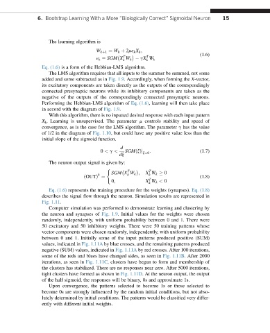
The learning algorithm is
W kþ1 ¼ W k þ 2me k X k ;
(1.6)
T T

e k ¼ SGM X W k gX W k
k k
Eq. (1.6) is a form of the Hebbian-LMS algorithm.
The LMS algorithm requires that all inputs to the summer be summed, not some
added and some subtracted as in Fig. 1.9. Accordingly, when forming the X-vector,
its excitatory components are taken directly as the outputs of the correspondingly
connected presynaptic neurons while its inhibitory components are taken as the
negative of the outputs of the correspondingly connected presynaptic neurons.
Performing the Hebbian-LMS algorithm of Eq. (1.6), learning will then take place
in accord with the diagram of Fig. 1.9.
With this algorithm, there is no inputted desired response with each input pattern
X k . Learning is unsupervised. The parameter m controls stability and speed of
convergence, as is the case for the LMS algorithm. The parameter g has the value
of 1/2 in the diagram of Fig. 1.10, but could have any positive value less than the
initial slope of the sigmoid function.
d
0 < g < SGMðxÞj x¼0 . (1.7)
dx
The neuron output signal is given by:
(
T T
SGM X W k ; X W k 0
k k k
ðOUTÞ ¼ T (1.8)
0; X W k < 0
k
Eq. (1.6) represents the training procedure for the weights (synapses). Eq. (1.8)
describes the signal flow through the neuron. Simulation results are represented in
Fig. 1.11.
Computer simulation was performed to demonstrate learning and clustering by
the neuron and synapses of Fig. 1.9. Initial values for the weights were chosen
randomly, independently, with uniform probability between 0 and 1. There were
50 excitatory and 50 inhibitory weights. There were 50 training patterns whose
vector components were chosen randomly, independently, with uniform probability
between 0 and 1. Initially some of the input patterns produced positive (SUM)
values, indicated in Fig. 1.11A by blue crosses, and the remaining patterns produced
negative (SUM) values, indicated in Fig. 1.11A by red crosses. After 100 iterations,
some of the reds and blues have changed sides, as seen in Fig. 1.11B. After 2000
iterations, as seen in Fig. 1.11C, clusters have begun to form and membership of
the clusters has stabilized. There are no responses near zero. After 5000 iterations,
tight clusters have formed as shown in Fig. 1.11D. At the neuron output, the output
of the half sigmoid, the responses will be binary, 0s and approximate 1s.
Upon convergence, the patterns selected to become 1s or those selected to
become 0s are strongly influenced by the random initial conditions, but not abso-
lutely determined by initial conditions. The patterns would be classified very differ-
ently with different initial weights.