Page 24 - Artificial Intelligence in the Age of Neural Networks and Brain Computing

5. Bootstrap Learning With a Sigmoidal Neuron 11

Weights

)
Xk (SUM k
Input  (OUT) k
Pattern
Vector
SIGMOID
g
Â
- +
ek
Error
FIGURE 1.7
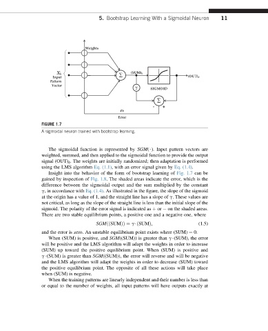
A sigmoidal neuron trained with bootstrap learning.

The sigmoidal function is represented by SGM($). Input pattern vectors are
weighted, summed, and then applied to the sigmoidal function to provide the output
signal (OUT) k . The weights are initially randomized; then adaptation is performed
using the LMS algorithm Eq. (1.1), with an error signal given by Eq. (1.4).
Insight into the behavior of the form of bootstrap learning of Fig. 1.7 can be
gained by inspection of Fig. 1.8. The shaded areas indicate the error, which is the
difference between the sigmoidal output and the sum multiplied by the constant
g, in accordance with Eq. (1.4). As illustrated in the figure, the slope of the sigmoid
at the origin has a value of 1, and the straight line has a slope of g. These values are
not critical, as long as the slope of the straight line is less than the initial slope of the
sigmoid. The polarity of the error signal is indicated as þ or on the shaded areas.
There are two stable equilibrium points, a positive one and a negative one, where
SGMððSUMÞÞ ¼ g$ðSUMÞ; (1.5)
and the error is zero. An unstable equilibrium point exists where (SUM) ¼ 0.
When (SUM) is positive, and SGM((SUM)) is greater than g$(SUM), the error
will be positive and the LMS algorithm will adapt the weights in order to increase
(SUM) up toward the positive equilibrium point. When (SUM) is positive and
g$(SUM) is greater than SGM((SUM)), the error will reverse and will be negative
and the LMS algorithm will adapt the weights in order to decrease (SUM) toward
the positive equilibrium point. The opposite of all these actions will take place
when (SUM) is negative.
When the training patterns are linearly independent and their number is less than
or equal to the number of weights, all input patterns will have outputs exactly at