Page 19 - Artificial Intelligence in the Age of Neural Networks and Brain Computing

6 CHAPTER 1 Nature’s Learning Rule: The Hebbian-LMS Algorithm

Weights
x k 1 w k 1
Summer
x k 2 w k 2
(SUM) k + 1 q k
k X x k 3 w k 3 Â − 1 Output

Input
Signum
Pa ern
x nk w nk
Vector
Â
– +
e k d = q k
k
Error
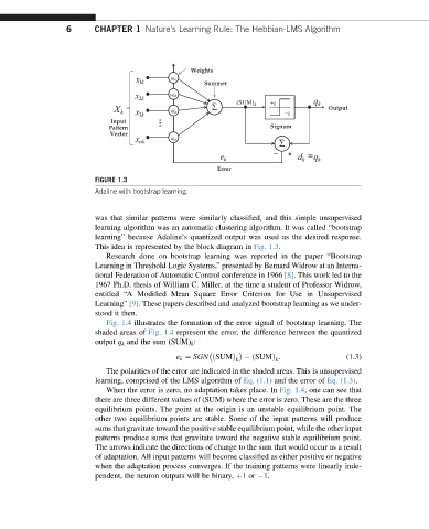
FIGURE 1.3
Adaline with bootstrap learning.

was that similar patterns were similarly classified, and this simple unsupervised
learning algorithm was an automatic clustering algorithm. It was called “bootstrap
learning” because Adaline’s quantized output was used as the desired response.
This idea is represented by the block diagram in Fig. 1.3.
Research done on bootstrap learning was reported in the paper “Bootstrap
Learning in Threshold Logic Systems,” presented by Bernard Widrow at an Interna-
tional Federation of Automatic Control conference in 1966 [8]. This work led to the
1967 Ph.D. thesis of William C. Miller, at the time a student of Professor Widrow,
entitled “A Modified Mean Square Error Criterion for Use in Unsupervised
Learning” [9]. These papers described and analyzed bootstrap learning as we under-
stood it then.
Fig. 1.4 illustrates the formation of the error signal of bootstrap learning. The
shaded areas of Fig. 1.4 represent the error, the difference between the quantized
output q k and the sum (SUM) k :

e k ¼ SGN ðSUMÞ ðSUMÞ . (1.3)
k k
The polarities of the error are indicated in the shaded areas. This is unsupervised
learning, comprised of the LMS algorithm of Eq. (1.1) and the error of Eq. (1.3).
When the error is zero, no adaptation takes place. In Fig. 1.4, one can see that
there are three different values of (SUM) where the error is zero. These are the three
equilibrium points. The point at the origin is an unstable equilibrium point. The
other two equilibrium points are stable. Some of the input patterns will produce
sums that gravitate toward the positive stable equilibrium point, while the other input
patterns produce sums that gravitate toward the negative stable equilibrium point.
The arrows indicate the directions of change to the sum that would occur as a result
of adaptation. All input patterns will become classified as either positive or negative
when the adaptation process converges. If the training patterns were linearly inde-
pendent, the neuron outputs will be binary, þ1or 1.