Page 23 - Artificial Intelligence in the Age of Neural Networks and Brain Computing

10 CHAPTER 1 Nature’s Learning Rule: The Hebbian-LMS Algorithm

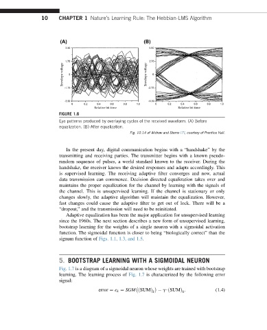
FIGURE 1.6
Eye patterns produced by overlaying cycles of the received waveform. (A) Before
equalization. (B) After equalization.
Fig. 10.14 of Widrow and Sterns [7], courtesy of Prentice Hall.

In the present day, digital communication begins with a “handshake” by the
transmitting and receiving parties. The transmitter begins with a known pseudo-
random sequence of pulses, a world standard known to the receiver. During the
handshake, the receiver knows the desired responses and adapts accordingly. This
is supervised learning. The receiving adaptive filter converges and now, actual
data transmission can commence. Decision directed equalization takes over and
maintains the proper equalization for the channel by learning with the signals of
the channel. This is unsupervised learning. If the channel is stationary or only
changes slowly, the adaptive algorithm will maintain the equalization. However,
fast changes could cause the adaptive filter to get out of lock. There will be a
“dropout,” and the transmission will need to be reinitiated.
Adaptive equalization has been the major application for unsupervised learning
since the 1960s. The next section describes a new form of unsupervised learning,
bootstrap learning for the weights of a single neuron with a sigmoidal activation
function. The sigmoidal function is closer to being “biologically correct” than the
signum function of Figs. 1.1, 1.3, and 1.5.

5. BOOTSTRAP LEARNING WITH A SIGMOIDAL NEURON
Fig. 1.7 is a diagram of a sigmoidal neuron whose weights are trained with bootstrap
learning. The learning process of Fig. 1.7 is characterized by the following error
signal:

error ¼ e k ¼ SGM ðSUMÞ g$ðSUMÞ . (1.4)
k k