Page 18 - Artificial Intelligence in the Age of Neural Networks and Brain Computing

3. Unsupervised Learning With Adaline, From the 1960s 5

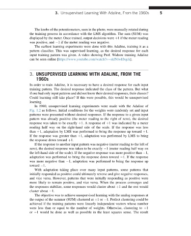
The knobs of the potentiometers, seen in the photo, were manually rotated during
the training process in accordance with the LMS algorithm. The sum (SUM) was
displayed by the meter. Once trained, output decisions were þ1 if the meter reading
was positive, and 1 if the meter reading was negative.
The earliest learning experiments were done with this Adaline, training it as a
pattern classifier. This was supervised learning, as the desired response for each
input training pattern was given. A video showing Prof. Widrow training Adaline
can be seen online [https://www.youtube.com/watch?v¼skfNlwEbqck].

3. UNSUPERVISED LEARNING WITH ADALINE, FROM THE
1960s
In order to train Adaline, it is necessary to have a desired response for each input
training pattern. The desired response indicated the class of the pattern. But what
if one had only input patterns and did not know their desired responses, their classes?
Could learning still take place? If this were possible, this would be unsupervised
learning.
In 1960, unsupervised learning experiments were made with the Adaline of
Fig. 1.2 as follows. Initial conditions for the weights were randomly set and input
patterns were presented without desired responses. If the response to a given input
pattern was already positive (the meter reading to the right of zero), the desired
response was taken to be exactly þ1. A response of þ1 was indicated by a meter
reading half way on the right-hand side of the scale. If the response was less
than þ1, adaptation by LMS was performed to bring the response up toward þ1.
If the response was greater than þ1, adaptation was performed by LMS to bring
the response down toward þ1.
If the response to another input pattern was negative (meter reading to the left of
zero), the desired response was taken to be exactly 1 (meter reading half way on
the left-hand side of the scale). If the negative response was more positive than 1,
adaptation was performed to bring the response down toward 1. If the response
was more negative than 1, adaptation was performed to bring the response up
toward 1.
With adaptation taking place over many input patterns, some patterns that
initially responded as positive could ultimately reverse and give negative responses,
and vice versa. However, patterns that were initially responding as positive were
more likely to remain positive, and vice versa. When the process converges and
the responses stabilize, some responses would cluster about þ1 and the rest would
cluster about 1.
The objective was to achieve unsupervised learning with the analog responses at
the output of the summer (SUM) clustered at þ1or 1. Perfect clustering could be
achieved if the training patterns were linearly independent vectors whose number
were less than or equal to the number of weights. Otherwise, clustering to þ1
or 1 would be done as well as possible in the least squares sense. The result