Page 16 - Artificial Intelligence in the Age of Neural Networks and Brain Computing

2. ADALINE and the LMS Algorithm, From the 1950s 3

The Hebbian-LMS algorithm will have engineering applications, and it may provide
insight into learning in living neural networks.
The current thinking that led us to the Hebbian-LMS algorithm has its roots in a
series of discoveries that were made since Hebb, from the late 1950s through the
1960s. These discoveries are reviewed in the next three sections. The sections
beyond describe Hebbian-LMS and how this algorithm could be nature’s algorithm
for learning at the neuron and synapse level.

2. ADALINE AND THE LMS ALGORITHM, FROM THE 1950s
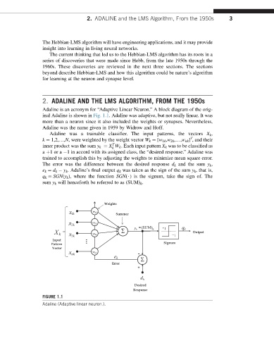
Adaline is an acronym for “Adaptive Linear Neuron.” A block diagram of the orig-
inal Adaline is shown in Fig. 1.1. Adaline was adaptive, but not really linear. It was
more than a neuron since it also included the weights or synapses. Nevertheless,
Adaline was the name given in 1959 by Widrow and Hoff.
Adaline was a trainable classifier. The input patterns, the vectors X k ,
T
k ¼ 1,2,.,N, were weighted by the weight vector W k ¼ [w 1k ,w 2k ,.,w nk ] , and their
T
inner product was the sum y k ¼ X W k . Each input pattern X k was to be classified as
k
a þ1ora 1 in accord with its assigned class, the “desired response.” Adaline was
trained to accomplish this by adjusting the weights to minimize mean square error.
The error was the difference between the desired response d k and the sum y k ,
e k ¼ d k y k . Adaline’s final output q k was taken as the sign of the sum y k , that is,
q k ¼ SGN(y k ), where the function SGN($) is the signum, take the sign of. The
sum y k will henceforth be referred to as (SUM) k .

Weights
w
k x 1 k 1 Summer
w
k x 2 k 2 k y = (SUM) + k q
X k k x 3 w k 3 Â k 1 − 1 Output

Input
Pattern Signum
Vector
nk x w nk -
k e
Â
Error
+
k d
Desired
Response
FIGURE 1.1
Adaline (Adaptive linear neuron.).