Page 17 - Artificial Intelligence in the Age of Neural Networks and Brain Computing

4 CHAPTER 1 Nature’s Learning Rule: The Hebbian-LMS Algorithm

The weights of Adaline were trained with the LMS algorithm, as follows:
W kþ1 ¼ W k þ 2me k X k ; (1.1)
T
e k ¼ d k X W k . (1.2)
k
Averaged over the set of training patterns, the mean square error is a quadratic
function of the weights, a quadratic “bowl.” The LMS algorithm uses the methodol-
ogy of steepest descent, a gradient method, for pulling the weights to the bottom of
the bowl, thus minimizing mean square error.
The LMS algorithm was invented by Widrow and Hoff in 1959 [6], 10 years after
the publication of Hebb’s seminal book. The derivation of the LMS algorithm is
given in many references. One such reference is the book Adaptive Signal Process-
ing by Widrow and Stearns [7]. The LMS algorithm is the most widely used learning
algorithm in the world today. It is used in adaptive filters that are key elements in all
modems, for channel equalization and echo canceling. It is one of the basic technol-
ogies of the Internet and of wireless communications. It is basic to the field of digital
signal processing.
The LMS learning rule is quite simple and intuitive. Eqs. (1.1) and (1.2) can be
represented in words:
“With the presentation of each input pattern vector and its associated desired
response, the weight vector is changed slightly by adding the pattern vector to
the weight vector, making the sum more positive, or subtracting the pattern vector
from the weight vector, making the sum more negative, changing the sum in
proportion to the error in a direction to make the error smaller.”

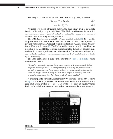
A photograph of a physical Adaline made by Widrow and Hoff in 1960 is shown
in Fig. 1.2. The input patterns of this Adaline were binary, 4 4 arrays of pixels,
each pixel having a value of þ1or 1, set by the 4 4 array of toggle switches.
Each toggle switch was connected to a weight, implemented by a potentiometer.

FIGURE 1.2
Knobby Adaline.