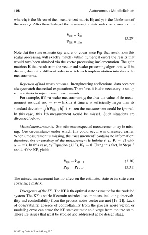
Page 125 - Autonomous Mobile Robots
P. 125
108                                    Autonomous Mobile Robots

                                where h i is the ith row of the measurement matrix H k and y i is the ith element of
                                thevectory. After the mth step oftherecursion, thestateand errorcovarianceare

                                                            ˆ x k|k = ˆ x m
                                                                                          (3.29)
                                                            P k|k = p m

                                Note that the state estimate ˆ x k|k and error covariance P k|k that result from this
                                scalar processing will exactly match (within numerical error) the results that
                                would have been obtained via the vector processing implementation. The gain
                                matrices K that result from the vector and scalar processing algorithms will be
                                distinct, due to the different order in which each implementation introduces the
                                measurements.

                                   Rejection of bad measurements. In engineering applications, data does not
                                always match theoretical expectations. Therefore, it is also necessary to set up
                                some criteria to reject some measurements.
                                   For example, if for a scalar measurement y i the absolute value of the meas-
                                urement residual res i = y i − h i ˆ x i−1 at time k is sufficiently larger than its

                                                         T
                                standard deviation  h i P k|k−1 h + r, then the measurement could be ignored.
                                                         i
                                In this case, this kth measurement would be missed. Such situations are
                                discussed below.
                                   Missed measurements. Sometimes an expected measurement may be miss-
                                ing. One circumstance under which this could occur was discussed earlier.
                                When a measurement is missing, the “measurement” contains no information;
                                therefore, the uncertainty of the measurement is infinite (i.e., R = αI with
                                α =∞). In this case, by Equation (3.23), K k = 0. Using this fact, in Steps 3
                                and 4 of the KF, yields


                                                                                          (3.30)
                                                          ˆ x k|k = ˆ x k|k−1
                                                          P k|k = P k|k−1                 (3.31)

                                The missed measurement has no effect on the estimated state or its state error
                                covariance matrix.
                                   Divergence of the KF. The KF is the optimal state estimator for the modeled
                                system. The KF is stable if certain technical assumptions, including observab-
                                ility and controllability from the process noise vector are met [19–21]. Lack
                                of observability, absence of controllability from the process noise vector, or
                                modeling error can cause the KF state estimate to diverge from the true state.
                                These are issues that must be studied and addressed at the design stage.


                                 © 2006 by Taylor & Francis Group, LLC


                                FRANKL: “dk6033_c003” — 2006/3/31 — 16:42 — page 108 — #10

