Page 128 - Autonomous Mobile Robots

Data Fusion via Kalman Filter 111

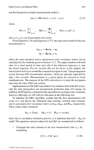
and the linearized (residual) measurement model is

δy(t) = H(t)δx(t) + v (t) + e y (t) (3.37)
where

∂f ∂h ∗
F(t) = , H(t) = , G(t) = g(x , t)
∂x x=x ∗ ∂x x=x ∗
and e x (t),e y (t) are linearization error terms.
From Equation (3.36) and Equation (3.37), the equivalent model for discrete
measurements is

δx k+1 = k δx k + w k
δy k = H k δx k + v k

where the state transition matrix and process noise covariance matrix can be
calculated by the methods given in Section 3.2.1. The approximation will hold
only for a short period of time and only if the reference trajectory is near
the actual trajectory. For the systems that are the focus of this chapter, the
linearizationwilloccuraroundthecomputednavigationstate. Timepropagation
occurs between GPS measurement epoches, which are typically separated by
only a few seconds. Measurements at a given epoch are assumed to occur
simultaneously. The purpose of the GPS corrections is to keep the navigation
state near the state of the true system.
Implementation ofthe EKF algorithm isvery similarto thatofthe KF,infact,
only the state propagation and measurement prediction steps will change. In
addition, the P matrices computed in the algorithm are no longer true covariance
matrices; although, we will still use that name in the following text.
To initialize the EKF algorithm, assume that the first measurement will
occur at t 1 and denote the initialized state estimate, residual state estimate,
and its associated error covariance matrix as ˆ x 0|0 , δˆ x 0|0 , and P 0|0 , respectively.
These initial values should be

ˆ x 0|0 = E(x 0 ), δˆ x 0|0 = 0, P 0|0 = cov(x 0 )

Since this is a nonlinear estimation process, it is important that x(0) − ˆ x 0|0 be
small. The equations and procedures for the EKF are summarized as follows:

1. Propagate the state estimate to the next measurement time t k+1 by
integrating
∗
∗
˙ x (t) = f(x , u, t) (3.38)

© 2006 by Taylor & Francis Group, LLC

FRANKL: “dk6033_c003” — 2006/3/31 — 16:42 — page 111 — #13