Page 44 - Autonomous Mobile Robots

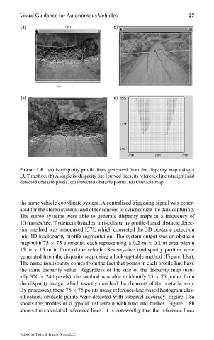
Visual Guidance for Autonomous Vehicles 27

(a) (b)

(c) (d)

FIGURE 1.8 (a) Isodisparity profile lines generated from the disparity map using a
LUT method. (b) A single isodisparity line (curved line), its reference line (straight) and
detected obstacle pixels. (c) Detected obstacle points. (d) Obstacle map.

the same vehicle coordinate system. A centralized triggering signal was gener-
ated for the stereo systems and other sensors to synchronize the data capturing.
The stereo systems were able to generate disparity maps at a frequency of
10 frames/sec. To detect obstacles, an isodisparity profile-based obstacle detec-
tion method was introduced [37], which converted the 3D obstacle detection
into 1D isodisparity profile segmentation. The system output was an obstacle
map with 75 × 75 elements, each representing a 0.2 m × 0.2 m area within
15 m × 15 m in front of the vehicle. Seventy-five isodisparity profiles were
generated from the disparity map using a look-up-table method (Figure 1.8a).
The name isodisparity comes from the fact that points in each profile line have
the same disparity value. Regardless of the size of the disparity map (usu-
ally 320 × 240 pixels), the method was able to identify 75 × 75 points from
the disparity image, which exactly matched the elements of the obstacle map.
By processing these 75 × 75 points using reference-line-based histogram clas-
sification, obstacle points were detected with subpixel accuracy. Figure 1.8a
shows the profiles of a typical test terrain with road and bushes. Figure 1.8b
shows the calculated reference lines. It is noteworthy that the reference lines

© 2006 by Taylor & Francis Group, LLC

FRANKL: “dk6033_c001” — 2006/3/31 — 16:42 — page 27 — #27