Page 153 - Basic Structured Grid Generation

142 Basic Structured Grid Generation

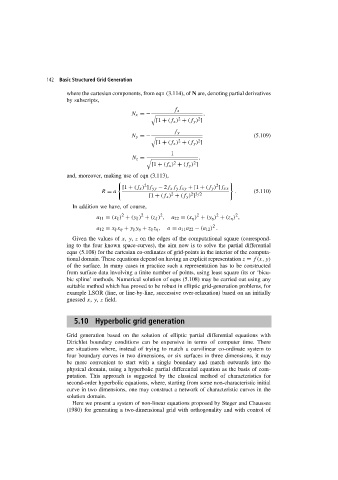
where the cartesian components, from eqn (3.114), of N are, denoting partial derivatives
by subscripts,

f x
,
N x =−#
2 2
[1 + (f x ) + (f y ) ]
f y
(5.109)
N y =−#
2 2
[1 + (f x ) + (f y ) ]
1
,
N z = #
2 2
[1 + (f x ) + (f y ) ]
and, moreover, making use of eqn (3.113),

2 2
[1 + (f x ) ]f yy − 2f x f y f xy +[1 + (f y ) ]f xx
R = a . (5.110)
2
2 3/2
[1 + (f x ) + (f y ) ]
In addition we have, of course,
2
2
2
2
2
2
a 11 = (x ξ ) + (y ξ ) + (z ξ ) , a 22 = (x η ) + (y η ) + (z η ) ,
2
a 12 = x ξ x η + y ξ y η + z ξ z η , a = a 11 a 22 − (a 12 ) .
Given the values of x, y, z on the edges of the computational square (correspond-
ing to the four known space-curves), the aim now is to solve the partial differential
eqns (5.108) for the cartesian co-ordinates of grid-points in the interior of the computa-
tional domain. These equations depend on having an explicit representation z = f (x, y)
of the surface. In many cases in practice such a representation has to be constructed
from surface data involving a finite number of points, using least square fits or ‘bicu-
bic spline’ methods. Numerical solution of eqns (5.108) may be carried out using any
suitable method which has proved to be robust in elliptic grid-generation problems, for
example LSOR (line, or line-by-line, successive over-relaxation) based on an initially
guessed x, y, z field.

5.10 Hyperbolic grid generation

Grid generation based on the solution of elliptic partial differential equations with
Dirichlet boundary conditions can be expensive in terms of computer time. There
are situations where, instead of trying to match a curvilinear co-ordinate system to
four boundary curves in two dimensions, or six surfaces in three dimensions, it may
be more convenient to start with a single boundary and march outwards into the
physical domain, using a hyperbolic partial differential equation as the basis of com-
putation. This approach is suggested by the classical method of characteristics for
second-order hyperbolic equations, where, starting from some non-characteristic initial
curve in two dimensions, one may construct a network of characteristic curves in the
solution domain.
Here we present a system of non-linear equations proposed by Steger and Chaussee
(1980) for generating a two-dimensional grid with orthogonality and with control of