Page 150 - Basic Structured Grid Generation

Differential models for grid generation 139

5.7.2 Numerical aspects

Weight function equation
Here we present a standard finite-difference scheme for solving eqn (5.83). The interval
0 ξ 1 is divided into m equal intervals, and we can label (m + 1) discrete points
ξ i = i ξ, i = 0, 1,. ..,m, with ξ = 1/m. It is useful to be able to evaluate certain
quantities at intermediate points, so that we have the finite-difference approximations
at the point corresponding to i:

d dx/dξ 1 dx/dξ dx/dξ
! "
− , (5.95)
dξ ϕ ξ ϕ 1 ϕ 1
i i+ i−
2 2
with
dx x i+1 − x i dx x i − x i−1

, (5.96)
dξ 1 ξ dξ 1 ξ
i+ i−
2 2
Then this finite-difference version of eqn (5.83) becomes

1 1 1 1 1
x i−1 − + x i + x i+1 = 0,
( ξ) 2 ϕ 1 ϕ 1 ϕ 1 ϕ 1
i− 2 i− 2 i+ 2 i+ 2
or
−a i x i−1 + b i x i − c i x i+1 = 0, i = 1, 2,..., (m − 1) , (5.97)

1 1 1 1
with a i = , b i = + , c i = , i = 1, 2,...,(m − 1). Note that
ϕ 1 ϕ 1 ϕ 1 ϕ 1
i− 2 i− 2 i+ 2 i+ 2
b i = a i + c i .
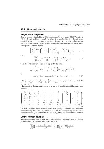
Incorporating the end-conditions x 0 = a, x m = b, we obtain the tridiagonal matrix
equation
     
b 1 −c 1 0 0 − – 0 x 1 a 1 a
 −a 2 b 2 −c 2 0 – – –   x 2   0 
 0 −a 3 b 3 −c 3 – – –     0 


  − 

 0 0 – – – – –     −  .


  −  = 
 − – – – – – 0   −   − 
     
     
− −− – 0 −a m−2 b m−2 −c m−2 − 0
0 – – 0 0 −a m−1 b m−1 x m−1 c m−1 b
(5.98)
The matrix of coefficients is also symmetric, since c i = a i+1 . Solutions may be obtained
efficiently using the Thomas Algorithm or SOR. On the accompanying disk the subdi-
rectory Book/one.d.gds contains the file line.SOR.f, which applies SOR to the problem.
Control function equation
A numerical scheme for solving eqn (5.80) is shown here. With the same uniform grid
as above along the computational ξ-axis, we have
d x x i+1 − 2x i + x i−1 and dx x i+1 − x i−1 ,
2
dξ 2 i ( ξ) 2 dξ i 2( ξ)