Page 146 - Basic Structured Grid Generation

Differential models for grid generation 135

k
k
y (x ,y ) y
P
P
(x k +1 ,y k +1 )
B P P
k
k
(x ,y ) P B P
B
B
k +1
k +1
(x B ,y B )
O O
x x
Before adjustment After adjustment
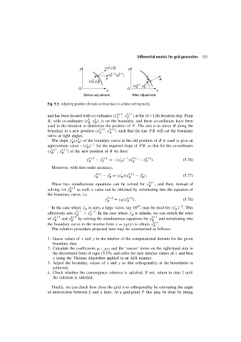
Fig. 5.5 Adjusting position of nodes on boundary to achieve orthogonality.
k+1 k+1
and has been located with co-ordinates (x ,y ) at the (k+1)th iteration step. Point
P P
k
k
B, with co-ordinates (x ,y ), is on the boundary, and these co-ordinates have been
B B
used in the iteration to determine the position of P . The aim is to move B along the
boundary to a new position (x k+1 ,y k+1 ) such that the line PB will cut the boundary
B B
curve at right angles.
k

The slope y (x ) of the boundary curve at the old position of B is used to give an
B B
−1
approximate value −(y ) for the required slope of PB, so that for the co-ordinates
B
(x k+1 ,y k+1 ) of the new position of B we have
B B
−1
y k+1 − y k+1 =−(y ) (x k+1 − x k+1 ). (5.76)
B P B B P
Moreover, with first-order accuracy,
k
k

y k+1 − y = (y )(x k+1 − x ). (5.77)
B B B B B
These two simultaneous equations can be solved for x k+1 , and then, instead of
B
k+1
solving for y as well, a value can be obtained by substituting into the equation of
B
the boundary curve, i.e.
k+1 k+1
y = y B (x ). (5.78)
B B
30
−1

In the case where y is zero, a large value, say 10 , may be used for (y ) .This
B B
k+1 k+1
effectively sets x B = x P . In the case where y is infinite, we can switch the roles
B
of x k+1 and y k+1 by solving the simultaneous equations for y k+1 and substituting into
B B B
k+1
the boundary curve in the inverse form x = x B (y) to obtain x .
B
The solution procedure proposed here may be summarized as follows:
1. Guess values of x and y in the interior of the computational domain for the given
boundary data.
2. Calculate the coefficients g 11 ,g 22 and the ‘source’ terms on the right-hand side in
the discretized form of eqns (5.19), and solve for new interior values of x and then
y using the Thomas Algorithm applied in an ADI manner.
3. Adjust the boundary values of x and y so that orthogonality at the boundaries is
achieved.
4. Check whether the convergence criterion is satisfied. If not, return to step 2 until
the criterion is satisfied.
Finally, we can check how close the grid is to orthogonality by estimating the angle
of intersection between ξ and η lines. At a grid-point P this may be done by fitting