Page 145 - Basic Structured Grid Generation

134 Basic Structured Grid Generation

j =5
j =4

j =3
j =2
j =1
i =1 i =2 i =3 i =4 i =5

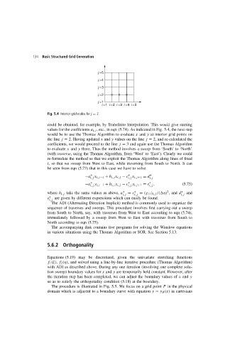
Fig. 5.4 Interior grid nodes for j = 2.

could be obtained, for example, by Transfinite Interpolation. This would give starting
values for the coefficients a i,j , etc., in eqn (5.74). As indicated in Fig. 5.4, the next step
would be to use the Thomas Algorithm to evaluate x and y at interior grid points on
the line j = 2. Having updated x and y values on the line j = 2, and re-calculated the
coefficients, we would proceed to the line j = 3 and again use the Thomas Algorithm
to evaluate x and y there. Thus the method involves a sweep from ‘South’ to ‘North’
(with traverse, using the Thomas Algorithm, from ‘West’ to ‘East’). Clearly we could
re-formulate the method so that we exploit the Thomas Algorithm along lines of fixed
i, so that we sweep from West to East, while traversing from South to North. It can
be seen from eqn (5.73) that in this case we have to solve

∗
∗
−a x i,j−1 + b i,j x i,j − c x i,j+1 = d ∗
i,j i,j i,j
∗
∗
∗
−a y i,j−1 + b i,j y i,j − c y i,j+1 = e , (5.75)
i,j i,j i,j
2
where b i,j take the same values as above, a ∗ = c ∗ = (g 11 ) i,j /( η) ,and d ∗ and
i,j i,j i,j
e ∗ are given by different expressions which can easily be found.
i,j
The ADI (Alternating Direction Implicit) method is commonly used to organize the
sequence of traverses and sweeps. This procedure involves first carrying out a sweep
from South to North, say, with traverses from West to East according to eqn (5.74),
immediately followed by a sweep from West to East with traverses from South to
North according to eqn (5.75).
The accompanying disk contains five programs for solving the Winslow equations
in various situations using the Thomas Algorithm or SOR. See Section 5.13.
5.6.2 Orthogonality

Equations (5.19) may be discretized, given the univariate stretching functions
f 1 (ξ), f 2 (η), and solved using a line-by-line iterative procedure (Thomas Algorithm)
with ADI as described above. During any one iteration (involving one complete solu-
tion sweep) boundary values for x and y are temporarily held constant. However, after
the iteration step has been completed, we can adjust the boundary values of x and y
so as to satisfy the orthogonality condition (5.18) at the boundary.
The procedure is illustrated in Fig. 5.5. We focus on a grid point P in the physical
domain which is adjacent to a boundary curve with equation y = y B (x) in cartesians