Page 144 - Basic Structured Grid Generation

Differential models for grid generation 133

2
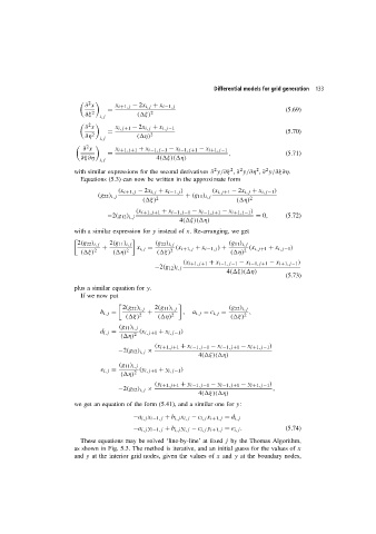
∂ x x i+1,j − 2x i,j + x i−1,j
= (5.69)
∂ξ 2 ( ξ) 2
i,j
2
∂ x x i,j+1 − 2x i,j + x i,j−1
= (5.70)
∂η 2 i,j ( η) 2
∂ x x i+1,j+1 + x i−1,j−1 − x i−1,j+1 − x i+1,j−1
2
= , (5.71)
∂ξ∂η i,j 4( ξ)( η)
2
2
2
2
2
with similar expressions for the second derivatives ∂ y/∂ξ ,∂ y/∂η ,∂ y/∂ξ∂η.
Equations (5.3) can now be written in the approximate form
(x i+1,j − 2x i,j + x i−1,j ) (x i,j+1 − 2x i,j + x i,j−1 )
(g 22 ) i,j 2 + (g 11 ) i,j 2
( ξ) ( η)
(x i+1,j+1 + x i−1,j−1 − x i−1,j+1 − x i+1,j−1 )
−2(g 12 ) i,j = 0, (5.72)
4( ξ)( η)
with a similar expression for y instead of x. Re-arranging, we get

2(g 22 ) i,j 2(g 11 ) i,j (g 22 ) i,j (g 11 ) i,j
+ x i,j = (x i+1,j + x i−1,j ) + (x i,j+1 + x i,j−1 )
( ξ) 2 ( η) 2 ( ξ) 2 ( η) 2
(x i+1,j+1 + x i−1,j−1 − x i−1,j+1 − x i+1,j−1 )
−2(g 12 ) i,j
4( ξ)( η)
(5.73)
plus a similar equation for y.
If we now put

2(g 22 ) i,j 2(g 11 ) i,j (g 22 ) i,j
b i,j = + , a i,j = c i,j = ,
( ξ) 2 ( η) 2 ( ξ) 2
(g 11 ) i,j
d i,j = (x i,j+1 + x i,j−1 )
( η) 2
(x i+1,j+1 + x i−1,j−1 − x i−1,j+1 − x i+1,j−1 )
−2(g 12 ) i,j ×
4( ξ)( η)
(g 11 ) i,j
e i,j = (y i,j+1 + y i,j−1 )
( η) 2
(y i+1,j+1 + y i−1,j−1 − y i−1,j+1 − y i+1,j−1 )
−2(g 12 ) i,j × ,
4( ξ)( η)
we get an equation of the form (5.41), and a similar one for y:

−a i,j x i−1,j + b i,j x i,j − c i,j x i+1,j = d i,j
−a i,j y i−1,j + b i,j y i,j − c i,j y i+1,j = e i,j . (5.74)
These equations may be solved ‘line-by-line’ at fixed j by the Thomas Algorithm,
as shown in Fig. 5.3. The method is iterative, and an initial guess for the values of x
and y at the interior grid nodes, given the values of x and y at the boundary nodes,