Page 147 - Basic Structured Grid Generation

136 Basic Structured Grid Generation

y
N
E
P
h W S
x

O
x
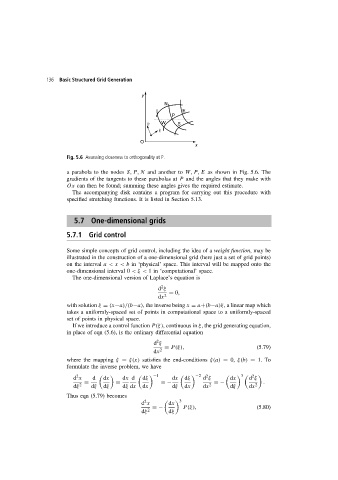
Fig. 5.6 Assessing closeness to orthogonality at P.

a parabola to the nodes S, P, N and another to W, P, E as shown in Fig. 5.6. The
gradients of the tangents to these parabolas at P and the angles that they make with
Ox can then be found; summing these angles gives the required estimate.
The accompanying disk contains a program for carrying out this procedure with
specified stretching functions. It is listed in Section 5.13.

5.7 One-dimensional grids

5.7.1 Grid control

Some simple concepts of grid control, including the idea of a weight function,may be
illustrated in the construction of a one-dimensional grid (here just a set of grid points)
on the interval a< x < b in ‘physical’ space. This interval will be mapped onto the
one-dimensional interval 0 <ξ < 1 in ‘computational’ space.
The one-dimensional version of Laplace’s equation is
2
d ξ
= 0,
dx 2
with solution ξ = (x−a)/(b−a), the inverse being x = a+(b−a)ξ, a linear map which
takes a uniformly-spaced set of points in computational space to a uniformly-spaced
set of points in physical space.
If we introduce a control function P(ξ), continuous in ξ, the grid generating equation,
in place of eqn (5.6), is the ordinary differential equation
2
d ξ
= P(ξ), (5.79)
dx 2
where the mapping ξ = ξ(x) satisfies the end-conditions ξ(a) = 0, ξ(b) = 1. To
formulate the inverse problem, we have
3
2
2
2
d x d dx dx d dξ −1 dx dξ −2 d ξ dx d ξ
= = =− =− .
dξ 2 dξ dξ dξ dx dx dξ dx dx 2 dξ dx 2
Thus eqn (5.79) becomes
2
d x dx 3
=− P(ξ), (5.80)
dξ 2 dξ