Page 143 - Basic Structured Grid Generation

132 Basic Structured Grid Generation

2. Obtain the generating system of equations for the Inverse Problem, with x, y as the
dependent variables and ξ, η as independent variables.
3. Discretize the generating equations using second-order accurate finite-difference
approximations.
4. Solve the resulting system of algebraic equations iteratively in the computational
plane subject to the given boundary conditions.

5.6.1 Thomas Algorithm

Here we show how to solve eqns (5.3) using the Thomas Algorithm. Because we have
a two-dimensional problem, the method has to be used in a ‘line-by-line’ fashion.
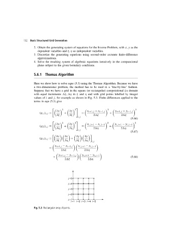
Suppose that we have a grid in the square (or rectangular) computational ξη domain
with equal increments ξ, η in ξ and η and with grid points labelled by integer
values of i and j, for example as shown in Fig. 5.3. Finite differences applied to the
terms in eqn (5.3) give

2 2 2 2
∂x ∂y x i+1,j − x i−1,j y i+1,j − y i−1,j
(g 11 ) i,j = + = +
∂ξ ∂ξ 2 ξ 2 ξ
i,j
(5.66)

2 2 2 2
∂x ∂y x i,j+1 − x i,j−1 y i,j+1 − y i,j−1
(g 22 ) i,j = + = +
∂η ∂η 2 η 2 η
i,j
(5.67)

∂x ∂x ∂y ∂y
(g 12 ) i,j = +
∂ξ ∂η ∂ξ ∂η
i,j

x i+1,j − x i−1,j x i,j+1 − x i,j−1
=
2 ξ 2 η

y i+1,j − y i−1,j y i,j+1 − y i,j−1
+ (5.68)
2 ξ 2 η

j =5

j =4
j =3
j =2

j =1
i =1 i =2 i =3 i =4 i =5
Fig. 5.3 Rectangular array of points.