Page 159 - Basic Structured Grid Generation

148 Basic Structured Grid Generation

5. A linear interpolation formula is now used to generate an improved value for ξ i ,
namely
ξ New − ξ i ξ i+1 − ξ i
i
= .
L 1 L 1 + L 2
which gives ξ New = ξ i + L 1 (ξ i+1 − ξ i ).
i L 1 +L 2
6. Having adjusted (in a loop) all the values of ξ i , we regenerate the two grids and
test again the value of ResMAT. The process is iterated until this value is within
the specified limit.

5.13 Website programs

5.13.1 Subdirectory: Book/Winslow.gds

This subdirectory contains six files. The first five solve the Winslow eqns (5.3) or the
Winslow equations with control functions (5.7) (TTM equations) for various planar
two-dimensional geometries, using either SOR or the Thomas Algorithm. They are:

1. W.SOR.f
2. W.adaptive.f
3. W.SOR.circle.f
4. W.adaptive.circle.f
5. W.trid.f
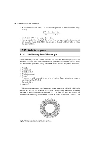
A number of grids obtained for domains of various shapes using these programs
are shown in Figs 5.7–5.12
The sixth file is
6. orthog.g.f

This program generates a two-dimensional planar orthogonal grid with grid-density
control by solving the Winslow eqns (5.19), incorporating univariate stretching
functions in both transformed co-ordinates ξ, η. The code has been written with the
possibility of employing finite-volume methods in mind, for example for solving the

Fig. 5.7 Grid generated employing Winslow equations.