Page 161 - Basic Structured Grid Generation

150 Basic Structured Grid Generation

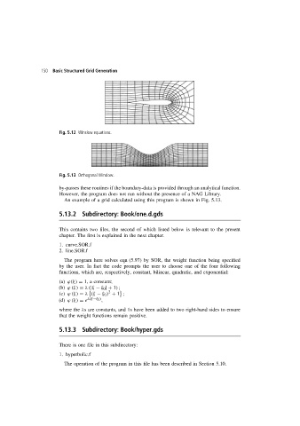
Fig. 5.12 Winslow equations.

Fig. 5.13 Orthogonal Winslow.

by-passes these routines if the boundary-data is provided through an analytical function.
However, the program does not run without the presence of a NAG Library.
An example of a grid calculated using this program is shown in Fig. 5.13.

5.13.2 Subdirectory: Book/one.d.gds

This contains two files, the second of which listed below is relevant to the present
chapter. The first is explained in the next chapter.
1. curve.SOR.f
2. line.SOR.f

The program here solves eqn (5.97) by SOR, the weight function being specified
by the user. In fact the code prompts the user to choose one of the four following
functions, which are, respectively, constant, bilinear, quadratic, and exponential:
(a) ϕ(ξ) = 1, a constant;
(b) ϕ (ξ) = λ (|ξ − ξ 0 | + 1) ;
2
$ %
(c) ϕ (ξ) = λ (ξ − ξ 0 ) + 1 ;
(d) ϕ (ξ) = e λ(ξ−ξ 0 ) ,
where the λs are constants, and 1s have been added to two right-hand sides to ensure
that the weight functions remain positive.

5.13.3 Subdirectory: Book/hyper.gds

There is one file in this subdirectory:
1. hyperbolic.f
The operation of the program in this file has been described in Section 5.10.