Page 182 - Basic Structured Grid Generation

Variational methods and adaptive grid generation 171

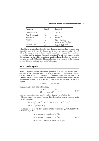
Functional Symbol Integrand
√
Orthogonality-3 I O,3 g 11 g 22
Area-Orthogonality I AO g 11 g 22
AO-squared I AO-squared (g 11 g 22 ) 2
√
Winslow I Win (g 11 + g 22 )/ g
2
2
Liao I li (g 11 ) + (g 22 ) + 2(g 12 ) 2
√ 2
Modified Liao I ml ([g 11 + g 22 ]/ g)
In all these variational problems the Euler-Lagrange equations lead to matrix equa-
tions of the form (6.48), in which the matrices A 11 , A 12 , A 22 are symmetric, with coef-
ficients depending at most on the first partial derivatives of the cartesian co-ordinates
x, y and the weight functions. The subdirectory Book/var.gds on the accompanying
disk contains five files which solve these equations. Each file offers two choices of
geometry, and both SOR and the Thomas Algorithm have been used in the numerical
solution. The files are listed at the end of this chapter.

6.4.8 Surface grids

A similar approach may be taken to the generation of a grid on a surface, such as
one given in the parametric form (3.3) with parameters u, v. Surface metric tensors
a αβ , as defined in eqn (3.17), and their determinants a, given by eqn (3.24), can be
used in place of g ij and g above. We assume that a surface can be mapped onto the
computational space 0 ξ 1, 0 η 1, and, indeed, we may seek the particular
mapping
u = u(ξ, η), v = v(ξ, η)
which minimizes some selected functional
√

H(a 11 ,a 22 ,a 12 , a)
I = dξ dη, (6.68)
{ϕ(u, v)} 2
where the weight function ϕ may be used for the purposes of adaptivity.
The metric tensor components here are defined according to the re-parameterization
r = r(ξ, η),sothat

2 2 2 2 2 2
a 11 = (x ξ ) + (y ξ ) + (z ξ ) , a 22 = (x η ) + (y η ) + (z η ) ,
a 12 = x ξ x η + y ξ y η + z ξ z η .

According to eqn (3.18), these are related to the components ˜a αβ with respect to the
parameters (u, v) by
2 2
a 11 = (u ξ ) ˜a 11 + 2u ξ v ξ ˜a 12 + (v ξ ) ˜a 22
2 2
a 22 = (u η ) ˜a 11 + 2u η v η ˜a 12 + (v η ) ˜a 22 (6.69)
a 12 = u ξ u η ˜a 11 + (u η v ξ + u ξ v η )˜a 12 + v ξ v η ˜a 22 .